Page 271 - Computational Fluid Dynamics for Engineers

References 261

8.5.3 Transition Prediction for Airfoil Flow

The procedure for determining the onset of transition location on an airfoil is
similar to the procedure used for the flat plate flow discussed in the previous
subsection. To demonstrate this, we consider an NACA 0012 airfoil at two chord
6
Reynolds numbers, R c = 10 6 and 3 x 10 . For the external velocity distribution
obtained from the HSPM computer program discussed in Section 6.5, the lami-
nar velocity profiles are computed with BLP for a = 0°, 2° and 4°. The neutral
stability calculations are then performed for each Reynolds number and angle of
attack. These calculations were then followed by amplification rate calculations
for each frequency computed on the neutral stability curve. For each calcula-
tion, the transition location is determined with respect to the surface distance
along the perimeter of the airfoil measured from the stagnation point and the
corresponding x/c location is calculated.
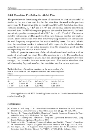
Table 8.2 presents a summary of the calculated transition locations at three
angles of attack and two chord Reynolds numbers for n — 8. The results show
that with increasing angle of attack, since the adverse pressure gradient becomes
stronger, the transition location moves upstream. The results also show that
with increasing Reynolds number, the transition location moves upstream.

Table 8.2. Onset of transition locations on the upper surface of an
NACA 0012 airfoil at two Reynolds numbers and three angles of
attack.
a 0° 2° 4°

Rc (s/c)tr-(x/c)tr (s / c)tr~(x / c)tr (s /' c) tr~(x /' 6) tr
1 x 10 6 0.505-0.49 0.33-0.31 0.16-0.13
3 x 10 6 0.355-0.34 0.21-0.19 0.10-0.075

More applications of STP, including its extension to three-dimensional flows
can be found in [3].

References

[1] Kleiser, L. and Zong, T.A.: "Numerical Simulation of Transition in Wall Bounded
Shear Flows," Annual Review of Fluid Mechanics, Vol. 23, pp. 495-538, 1991.
[2] Herbert, T.: "Parabolized Stability Equations," Special Course on Progress in Tran-
sition Modeling, AGARD Report 793, April 1994.
[3] Cebeci, T.: Stability and Transition: Theory and Application, Horizons Pub., Long
Beach, Calif, and Springer, Heidelberg, 2004.
[4] Smith, A.M.O.: "Transition, Pressure Gradient, and Stability Theory," Proceedings
IX International Congress of Applied Mechanics, Brussels, Vol. 4, pp. 234-2 4, 1956.
[5] Van Ingen, J.L.: "A Suggested Semi-empirical Method for the Calculation of the
Boundary-Layer Region," Report No. VTH71, VTH74, Delft, Holland, 1956.