Page 275 - Computational Fluid Dynamics for Engineers

9.2 Basic Concepts in Grid Generation and Mapping 265

(U) (U)
(U)
D C

A B

d,i) (1,1) (1.1)

X ° ' 2 3 ^
(a) (b)
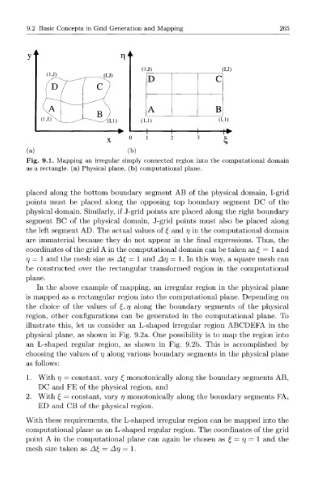
Fig. 9.1. Mapping an irregular simply connected region into the computational domain
as a rectangle, (a) Physical plane, (b) computational plane.

placed along the bottom boundary segment AB of the physical domain, I-grid
points must be placed along the opposing top boundary segment DC of the
physical domain. Similarly, if J-grid points are placed along the right boundary
segment BC of the physical domain, J-grid points must also be placed along
the left segment AD. The actual values of £ and rj in the computational domain
are immaterial because they do not appear in the final expressions. Thus, the
coordinates of the grid A in the computational domain can be taken as £ = 1 and
7] = 1 and the mesh size as A£ = 1 and Ar\ = 1. In this way, a square mesh can
be constructed over the rectangular transformed region in the computational
plane.
In the above example of mapping, an irregular region in the physical plane
is mapped as a rectangular region into the computational plane. Depending on
the choice of the values of £, 77 along the boundary segments of the physical
region, other configurations can be generated in the computational plane. To
illustrate this, let us consider an L-shaped irregular region ABCDEFA in the
physical plane, as shown in Fig. 9.2a. One possibility is to map the region into
an L-shaped regular region, as shown in Fig. 9.2b. This is accomplished by
choosing the values of 77 along various boundary segments in the physical plane
as follows:

1. With 77 = constant, vary £ monotonically along the boundary segments AB,
DC and FE of the physical region, and
2. With £ = constant, vary 77 monotonically along the boundary segments FA,
ED and CB of the physical region.
With these requirements, the L-shaped irregular region can be mapped into the
computational plane as an L-shaped regular region. The coordinates of the grid
point A in the computational plane can again be chosen as £ = 77 = 1 and the
mesh size taken as A£ = Arj = 1.