Page 280 - Computational Fluid Dynamics for Engineers

270 9. Grid Generation

(
XB1 =Zl(0> VB\ = 2/1 0 (9.4.4a)
and
%B2 = Z 2 (0> VB2 =2/2(0 (9.4.4b)
The range of £ in the computational plane is:

0 < £ < 1
and the transformation is defined so that at 77 = 0,

XBI = xi(0 = x(£, 0), y B1 = 2/1 (£) = 2/(f, 0) (9.4.5a)

and at 77 = 1,
XB2 = x 2(0 = x(£, 1), y B2 = 2/2 0 = 2/(f, 1) (9.4.5b)
(
A function defined on 0 < r? < 1 with parameters on the two boundaries com-
pletes the algebraic relation. This is chosen to be of the form

dX2
x = x(£,ri) = F l a ; i , — , . . . , 0 : 2 , (9.4.6a)
drj
dyi
dy2
y = y{i,r 1) = F[y l,—,...^ dr] (9.4.6b)
Smith and Weigel [2] suggest the use of either linear or cubic polynomials. For
a linear function, the relations in Eq. (9.4.6) become

x = (£){l - rj) + X2(S)v (9.4.7a)
Xl
V = 2/i(0(l -V) + V2(0V (9.4.7b)
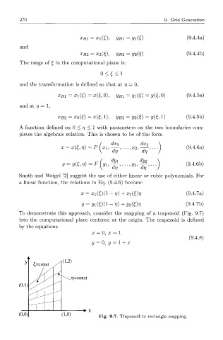
To demonstrate this approach, consider the mapping of a trapezoid (Fig. 9.7)
into the computational plane centered at the origin. The trapezoid is defined
by the equations
x = 0, x = 1
(9.4.8)
y = 0, y = l + x

T|=const
(0.1)

• X
(0,0)
Fig. 9.7. Trapezoid to rectangle mapping.