Page 277 - Computational Fluid Dynamics for Engineers

9.3 Stretched Grids 267

9.3 Stretched Grids

Let us assume that we are interested in the viscous flow solution of the conser-
vation equations on a body, where the velocity varies rapidly near the surface
of the physical plane. To calculate the details of this flow, a non-uniform grid,
which has fine spacing close to the surface and coarse spacing away from the
surface, is needed. To overcome the difficulties associated with the use of a non-
uniform grid, it is desirable to obtain the flow-field solution in the computational
plane where the grid is uniform (Fig. 9.4b) rather than in the physical plane
(Fig. 9.4a). We use the following coordinate transformation for this purpose,

(9.3.1a)
ln[A(y)}
77 = 1 - (9.3.1b)

Where:
P+{\-y/h) 0+1
A(y) = B = (9.3.2)
p-{l-y/hY 0-1
Here (3 is called the stretching parameter, which assumes values 1 < j3 < oo.
As f3 approaches unity, more grids are clustered near the wall in the physical
domain. The inverse transformation is:
(9.3.3a)
l
y_ ((3 + l)-((3-l)B -v
, „i (9.3.3b)
h
The continuity equation for steady flow in the two-dimensional physical plane,
see Eq. (2.2.12b), is
|
| : M + ( ^ = o

y k,
T
1
h—V 1

4
X
1
(a) (b)
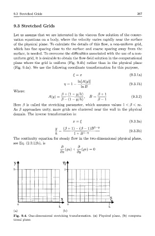
Fig. 9.4. One-dimensional stretching transformation, (a) Physical plane, (b) computa-
tional plane.