Page 278 - Computational Fluid Dynamics for Engineers

268 9. Grid Generation

In the computational plane, this equation can be written as
d Q(£ xu + £,yv) d Q(rj xu + r) yv)
d£ J dr] J
or, noting that the invariants of transformation are equal to zero,
r\ r\ r\ r\
0 (9.3.4)

The metrics in the above equation can be obtained from the transformation
given by Eq. (9.3.1),

2/? 1
6r = 1 , (,y = 0, r\ x = 0, rj y = 2 2 (9.3.5)
h.lnBp -(l-y/h)
Therefore, the form of the continuity equation in the computational plane, with
r\ y defined in Eq. (9.3.5) and with y in r\ y related to 7? by Eq. (9.3.3b) is:

0 (9.3.6)

Note that the transformed continuity equation retains its general form, except
for the coefficient r^-term. Therefore, the transformed equation (9.3.6) is slightly
more complicated than its original form, but it can now be solved for a uniform
grid. Once the solution is obtained in the computational domain, the results can
be transformed back to the physical domain with the inverse transformation
given by Eq. (9.3.3) for each (£, 77) location to the corresponding (x, y) location.

9.4 Algebraic Methods

The technique of using algebraic relations to cluster grid points close to the
surface can be extended to generate computational grids in two or three dimen-
sions, and to map arbitrary physical regions into a rectangular computational
domain.
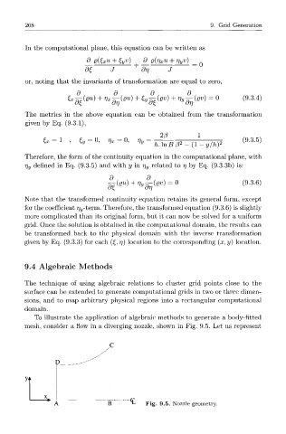
To illustrate the application of algebraic methods to generate a body-fitted
mesh, consider a flow in a diverging nozzle, shown in Fig. 9.5. Let us represent

B Fig. 9.5. Nozzle geometry.