Page 283 - Computational Fluid Dynamics for Engineers

9.4 Algebraic Methods 273

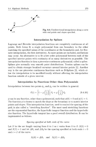
Fig. 9.9. Unidirectional interpolation along a curve
with end points and slopes specified.

Interpolation by Splines

Lagrange and Hermite interpolation functions are completely continuous at all
points. Both forms fit a single polynomial from one boundary to the other
matching the specified values of the coordinates at the boundaries and, for Her-
mite interpolation, the first derivatives. As more points are included, oscillations
may occur. An alternative is to fit a low order polynomial between each of the
specified interior points with continuity of as many derivatives as possible. The
interpolation function is then a piecewise-continuous polynomial, called a spline.
Splines give normally very smooth point distributions. Tension splines can be
used to obtain stronger localized curvature around interior points [1]. Another
way is the use piecewise continuous functions such as B-Splines [3], which al-
low the interpolation to be modified locally without affecting the interpolation
function outside of a given interval.

Interpolation by Functions Other than Polynomials
Interpolation between two points r x and r 2 can be written in general:

i
f(i) (9.4.16)
V ri+<p[j)r 2
*I
<fi can be any function, other than a polynomial, such that 0(0) = 0 and 0(1) = 1.
The function <\> is chosen to match the slope at the boundary or to match interior
points and slopes. This interpolation function, used to control the spacing of the
grid, is also called a "stretching function". The most used stretching functions
are the exponential function, the hyperbolic tangent function and the hyperbolic
sine function. The hyperbolic tangent has a good overall distribution. It can be
implemented as follows.

Spacing specified at both ends of the curve
Let S be the arc length varying from 0 to 1 as i varies from 0 to : S(0) = 0
/
and S(I) = 1 and let AS\ and AS 2 be the spacing specified at both ends i = 0
and i = / of the curve.

Si(0) = ASi and $ ( / ) - AS 2