Page 308 - Computational Fluid Dynamics for Engineers

298 10. Inviscid Compressible Flow

y*j
! Jy
n
l dSly^J?
/x/ dS2
n 2
Js '
y\*
— » >
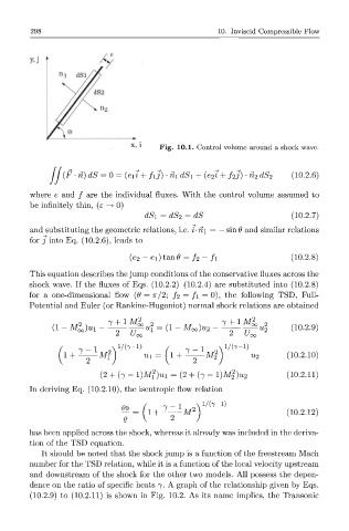
X, 1 Fig. 10.1. Control volume around a shock wave.

(F • ft) dS = 0 = (ei?+ ij) • m dSi + (e 2 ? + f 2j) • n 2 dS 2 (10.2.6)
/
/ /
where e and / are the individual fluxes. With the control volume assumed to
be infinitely thin, (e —> 0)
dSi = dS 2 = dS (10.2.7)

and substituting the geometric relations, i.e. i-n\ — — sin# and similar relations
for j into Eq. (10.2.6), leads to

( e 2 - e i ) t a u 0 = / 2 - / i (10.2.8)
This equation describes the jump conditions of the conservative fluxes across the
shock wave. If the fluxes of Eqs. (10.2.2)-(10.2.4) are substituted into (10.2.8)
for a one-dimensional flow (6 = 7r/2; / 2 = f\ = 0), the following TSD, Full-
Potential and Euler (or Rankine-Hugoniot) normal shock relations are obtained

(1 - Ml) Ul _ ! + ! * £ „ ? = (i - Moo)u 2 - X ± ^ . i (10.2.9)

7 _ 1 2 \ 1 / ( 7 - 1 } / 7 - 1 2 \ 1 / ( 7 - 1 }
1 + ^— Ml «! = ( ! + ^^Ml u 2 (10.2.10)
2 V V 2
2
(2 + (7 - l)M! )«i = (2 + (7 - l)Ml)u 2 (10.2.11)
In deriving Eq. (10.2.10), the isentropic flow relation

^ = ( l + ^ M 2 ) 1 / ( 7 _ 1 ) (10.2.12)

has been applied across the shock, whereas it already was included in the deriva-
tion of the TSD equation.
It should be noted that the shock jump is a function of the freest ream Mach
number for the TSD relation, while it is a function of the local velocity upstream
and downstream of the shock for the other two models. All possess the depen-
dence on the ratio of specific heats 7. A graph of the relationship given by Eqs.
(10.2.9) to (10.2.11) is shown in Fig. 10.2. As its name implies, the Transonic