Page 309 - Computational Fluid Dynamics for Engineers

10.3 Shock Capturing 299

1.00
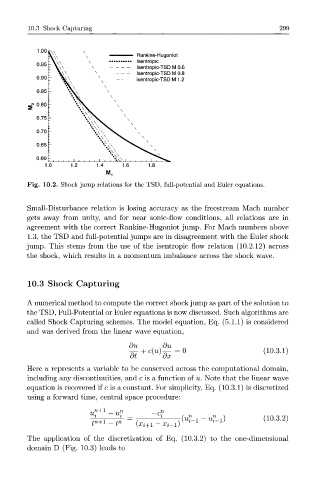
Rankine-Hugoniot
Isentropic
Isentropic-TSD M 0.6
Isentropic-TSD M 0.8
isentropic-TSD M 1.2

Fig. 10.2. Shock jump relations for the TSD, full-potential and Euler equations.

Small-Disturbance relation is losing accuracy as the freestream Mach number
gets away from unity, and for near sonic-flow conditions, all relations are in
agreement with the correct Rankine-Hugoniot jump. For Mach numbers above
1.3, the TSD and full-potential jumps are in disagreement with the Euler shock
jump. This stems from the use of the isentropic flow relation (10.2.12) across
the shock, which results in a momentum imbalance across the shock wave.

10.3 Shock Capturing

A numerical method to compute the correct shock jump as part of the solution to
the TSD, Full-Potential or Euler equations is now discussed. Such algorithms are
called Shock Capturing schemes. The model equation, Eq. (5.1.1) is considered
and was derived from the linear wave equation,

du .du
(10.3.1)

Here u represents a variable to be conserved across the computational domain,
including any discontinuities, and c is a function of u. Note that the linear wave
equation is recovered if c is a constant. For simplicity, Eq. (10.3.1) is discretized
using a forward time, central space procedure:

u^ 1 - c -
jn+1 _ n W + l i+1 XU) (10.3.2)
t
The application of the discretization of Eq. (10.3.2) to the one-dimensional
domain D (Fig. 10.3) leads to