Page 313 - Computational Fluid Dynamics for Engineers

10.5 Model Problem for the Transonic Small Disturbance Equation 303

10.5.1 Discretized Equation

The non-conservative two-dimensional TSD equation [Eq. (10.4.2)] is discretized
with the boundary conditions given by Eqs. (10.5.1)-(10.5.5) on a Cartesian
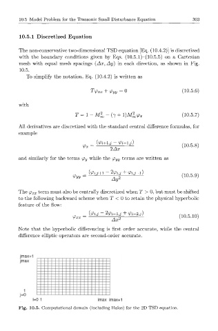
mesh with equal mesh spacings (Ax, Ay) in each direction, as shown in Fig.
10.5.
To simplify the notation, Eq. (10.4.2) is written as

T(fxx + ¥>yy = 0 (10.5.6)

with
T = 1 - Ml - (j + l)Ml<p x (10.5.7)

All derivatives are discretized with the standard central difference formulas, for
example

( 1 0 5 8 )
^ " 2Ax - -
and similarly for the terms cp y while the (p yy terms are written as

(<Pij+l ~ tyij + <£i,j-l)
Pyy 2 (10.5.9)
Ay

The ip xx term must also be centrally discretized when T > 0, but must be shifted
to the following backward scheme when T < 0 to retain the physical hyperbolic
feature of the flow:
(<Pij - 2<Pi-lj + <Pi-2, :
^Pxx — 2 (10.5.10)
Ax
Note that the hyperbolic differencing is first order accurate, while the central
difference elliptic operators are second-order accurate.

jmax+1
jmax

1
j=0
i=0 1 imax imax+1
Fig. 10.5. Computational domain (including Halos) for the 2D TSD equation.