Page 314 - Computational Fluid Dynamics for Engineers

304 10. Inviscid Compressible Flow

10.5.2 Solution Procedure and Sample Calculations

The computer program is given in Appendix B. First, a 2-D grid with equidistant
spacing is generated on the computational domain (i — 1 to imax, j = 1 to
jmax). The subroutine also generates the halo cells around the perimeter of
the computational grid (i = 0, i = imax + 1, j = 0 and j — jmax + 1 lines) for
reasons which will be discussed below.
The solution is initialized to a zero perturbation state (ip = 0) everywhere
and the boundary conditions are applied immediately, as will be discussed
shortly. Applying the ADI method discussed in subsection 4.5.2 in the y-
direction and sweeping the domain explicitly in the ^-direction, the discretized
Eq. (10.5.4) can be written in the form:

apij-i + btpij + c<pij+i = RHS (10.5.11)

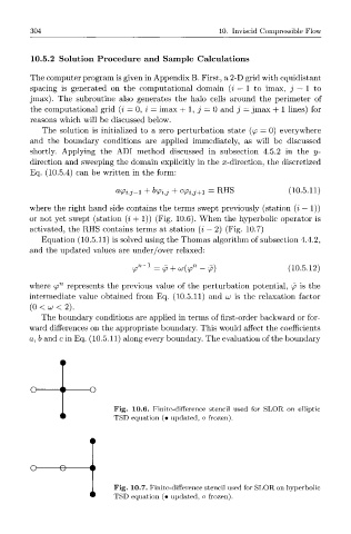
where the right hand side contains the terms swept previously (station (i — 1))
or not yet swept (station (i + 1)) (Fig. 10.6). When the hyperbolic operator is
activated, the RHS contains terms at station (i — 2) (Fig. 10.7)
Equation (10.5.11) is solved using the Thomas algorithm of subsection 4.4.2,
and the updated values are under /over relaxed:
.71+1 n
^ = ip + u((p - (f) (10.5.12)
where ip n represents the previous value of the perturbation potential, ip is the
intermediate value obtained from Eq. (10.5.11) and UJ is the relaxation factor
( 0 < C J < 2 ) .
The boundary conditions are applied in terms of first-order backward or for-
ward differences on the appropriate boundary. This would affect the coefficients
a, b and c in Eq. (10.5.11) along every boundary. The evaluation of the boundary

O -O

Fig. 10.6. Finite-difference stencil used for SLOR on elliptic
TSD equation (• updated, o frozen).

o- -e-

Fig. 10.7. Finite-difference stencil used for SLOR on hyperbolic
TSD equation (• updated, o frozen).