Page 372 - Computational Fluid Dynamics for Engineers

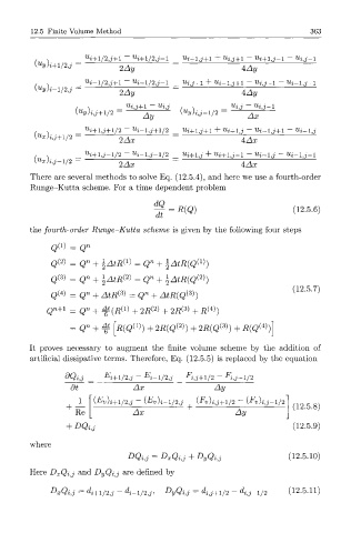
12.5 Finite Volume Method 363

L _ u
i+l/2,j+l i+l/2,j-l _ Ui+ij+i + Uij+i - Uj+ij-i - Uij-i
(%)i+l/2,j —
2Ay 4Ay
u
u i-l/2,j+l - i-l/2,j-l _ Uij+i + Ui-ij + i - Uij-i - Ui-ij-i
u
( y)i-l/2j =
2Ay 4Ay
l u
y)i,j+i/2 ~ ^ K y)i,j-i/2
Ax
/ x _ ^ + l , j + l / 2 ~ ^i-lJ+1/2 _ ^ i + l j + l + ^ i + l j ~ ^2-l,j+l ~ ^z-l,j

u
/ x _ u i+lj-l/2 ~ i-l,j-l/2 _ Ui+ij + U i + i j - i - Ui-ij - TXz—l,j —1
^ ^ « - V 2 " ^ x " lA~x
There are several methods to solve Eq. (12.5.4), and here we use a fourth-order
Runge-Kutta scheme. For a time dependent problem

= R(Q) (12.5.6)
dt
the fourth-order Runge-Kutta scheme is given by the following four steps

Q(2) = Qn + ^ AtRW =Qn + ^AtR(Q^)

Q(3) = Qn + l AtR(2) = Qn + ^AtR(Q^)
(12.5.7)
4
Q( ) = Q n + AtRW =Q n + AtR(QW)
Qn+1 =Qn + AL( R(1) + 2ij(2) + 2ij(3) + ijW)
n
4
(2
(3)
{1)
= Q + f [R(Q ) + 2i?(g ') + 2i?(Q ) + i?(Q< ))
It proves necessary to augment the finite volume scheme by the addition of
artificial dissipative terms. Therefore, Eq. (12.5.5) is replaced by the equation
dQ i,J _ E i+l/2,j - E i-l/2,j _ Fjj+1/2 - Fj,j-l/2
dt Ax Ay
E
E
1 ( v)i+l/2,j — ( v)i-l/2,j { v)i,j+l/2 - ( v)i,j-l/2
E
E
+ (12.5.8)
Re" Ax Ay
+ DQij (12.5.9)
where
(12.5.10)
Here D xQij and D yQij are defined by

D xQij = d i+i/ 2j — d i_ 1/ 2j, DyQij = dij+i/2 — d ij_ 1/ 2 (12.5.11)