Page 52 - Computational Fluid Dynamics for Engineers

1.5 Aerodynamics of Ground-Based Vehicles 37

of turbulence models (Chapter 3, [15,16]). Much work remains to be done in
the calibration and tailoring of turbulence models for vehicle application before
results of consistent accuracy can be obtained.
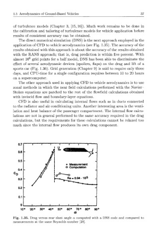
The direct numerical simulation (DNS) is the next approach employed in the
application of CFD to vehicle aerodynamics (see Fig. 1.35). The accuracy of the
results obtained with this approach is about the accuracy of the results obtained
with the RANS approach; that is, drag prediction is within five percent. With
almost 10 6 grid points for a half model, DNS has been able to discriminate the
effect of several aerodynamic devices (spoilers, flaps) on the drag and lift of a
sports car (Fig. 1.36). Grid generation (Chapter 9) is said to require only three
days, and CPU-time for a single configuration requires between 10 to 20 hours
on a supercomputer.
The other approach used in applying CFD to vehicle aerodynamics is to use
zonal methods in which the near field calculations performed with the Navier-
Stokes equations are patched to the rest of the flowfield calculations obtained
with inviscid flow and boundary-layer equations.
CFD is also useful in calculating internal flows such as in ducts connected
to the radiator and air conditioning units. Another interesting area is the venti-
lation and heat balance of the passenger compartment. The internal flow calcu-
lations are not in general performed to the same accuracy required in the drag
calculations, but the requirements for these calculations cannot be relaxed too
much since the internal flow produces its own drag component.

0.1

10° 20* 30° 40° 50° 60° 70° 80° 90°
a
Fig. 1.35. Drag versus rear slant angle a computed with a DNS code and compared to
measurements at the same Reynolds number [29].