Page 96 - Computational Fluid Dynamics for Engineers

82 3. Turbulence Models

modeling and are still used for many flows. Note that these are merely defini-
tions of £ and £ m: the assumption is that they will vary more slowly or more
simply than the shear stress and therefore be easier to correlate empirically.
Their names imply an analogy between turbulent motion and the molecular
motion that leads to viscous stresses, but this is now recognized as completely
misleading.
The specification of £ m or £ may be made in terms of algebraic equations
or in terms of a combination of algebraic and differential equations and this
has given rise to terminology involving the number of differential equations.
Thus, the closures may be described in terms of zero, one and two differential
equations. For a two-dimensional boundary-layer, the zero-equation approach
usually treats a turbulent boundary layer as a composite layer with separate
expressions for s m or £ in each region. The Cebeci-Smith (CS) model discussed
in detail in [2,3] and briefly in Section 3.2 is a typical example for this approach.
In the one-differential-equation approach the eddy viscosity is written, with
C/j denoting a constant, as
l 2
em = c^k / £ (3.1.3)
with k obtained from a differential equation which represents the transport of
turbulence energy and £ from an algebraic formula. The Spalart-Allmaras (SA)
model discussed in detail in [1-3, 9] and briefly in Section 3.3 is a good, useful
model that uses this approach.
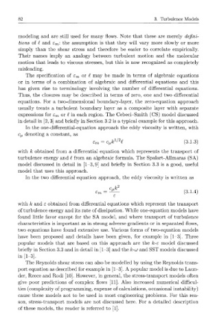
In the two differential equation approach, the eddy viscosity is written as

with k and e obtained from differential equations which represent the transport
of turbulence energy and its rate of dissipation. While one-equation models have
found little favor except for the SA model, and where transport of turbulence
characteristics is important as in strong adverse gradients or in separated flows,
two equations have found extensive use. Various forms of two-equation models
have been proposed and details have been given, for example in [1-3]. Three
popular models that are based on this approach are the k-e model discussed
briefly in Section 3.3 and in detail in [1-3] and the k-uj and SST models discussed
in [1-3].
The Reynolds shear stress can also be modelled by using the Reynolds trans-
port equation as described for example in [1-3]. A popular model is due to Laun-
der, Reece and Rodi [10]. However, in general, the stress-transport models often
give poor predictions of complex flows [11]. Also increased numerical difficul-
ties (complexity of programming, expense of calculations, occasional instability)
cause these models not to be used in most engineering problems. For this rea-
son, stress-transport models are not discussed here. For a detailed description
of these models, the reader is referred to [1].