Page 99 - Computational Fluid Dynamics for Engineers

3.2 Zero-Equation Models 85

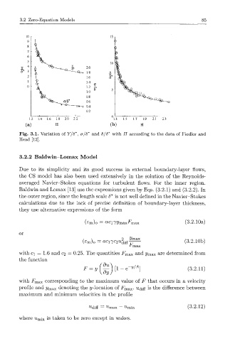
Fig. 3.1. Variation of Y/8*, a/8* and 8/8* with H according to the data of Fiedler and
Head [12].

3.2.2 Baldwin-Lomax Model

Due to its simplicity and its good success in external boundary-layer flows,
the CS model has also been used extensively in the solution of the Reynolds-
averaged Navier-Stokes equations for turbulent flows. For the inner region.
Baldwin and Lomax [13] use the expressions given by Eqs. (3.2.1) and (3.2.2). In
the outer region, since the length scale 6* is not well defined in the Navier-Stokes
calculations due to the lack of precise definition of boundary-layer thickness,
they use alternative expressions of the form

(£m)o = aci7y m a x F m a x (3.2.10a)

or
/ \ 2 2/max
(£m)o = aci7c 2 u diff — (3.2.10b)
with c\ — 1.6 and c 2 = 0.25. The quantities F m a x and ?/max are determined from
the function
, - , ( * ) [ ! - . - . * , (3.2.11)

with F m a x corresponding to the maximum value of F that occurs in a velocity
profile and y max denoting the y-location of F m a x . ^^iff is the difference between
maximum and minimum velocities in the profile

^diff — w max ^min (3.2.12)
where u m[ n is taken to be zero except in wakes.