Page 188 - Computational Statistics Handbook with MATLAB

Chapter 5: Exploratory Data Analysis 175

(
(
–
1
Θ T ) = Φ [ F T )]
1
1
(
(
1
–
Θ T 2 ) = Φ [ F T 2 )] (5.18)
,
(
,
Θ T i ) = T i ; i = 3 … d ,
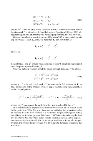
where Φ – 1 is the inverse of the standard normal cumulative distribution
function and is a function defined below (see Equations 5.19 and 5.20). We
F
see from Equation 5.18, that we will be changing only the first two rows of T.
We now describe the transformation of Equation 5.18 in more detail, work-
ing only with T 1 and T 2 . First, we note that T 1 can be written as
*
*
α
α
,
,
,
T 1 = ( z 1 … z j , … z n α * , )
as
and T 2
*
*
β
β
,
,
T = ( z , … z , … z β n * . )
1
2
j
α * β *
Recall that z j and z j would be coordinates of the j-th observation projected
onto the plane spanned by α β,( * * . )
γ
Next, we define a rotation about the origin through the angle as follows
˜ 1 t() 1 t() 2 t() γ
z j = z j cos γ + z j sin
(5.19)
˜ 2 t() 2 t() 1 t()
z j = z j cos γ – z j sin γ,
⁄
,
,
,
⁄
⁄
where γ = 0 π 4 π 8 3π 8 and z j 1 t() represents the j-th element of T 1 at
the t-th iteration of the process. We now apply the following transformation
to the rotated points,
– 
– 
1 rz j ) –
–
(
(
1 t + 1) Φ  ( ˜ 1 t() ) 0.5  2 t + 1) Φ  ( ˜ 2 t() 0.5  , 
1 rz j
z j = ------------------------------  z j = ------------------------------ (5.20)
 n   n 
1 t()
(
where rz j ) represents the rank (position in the ordered list) of z j 1 t() .
˜
˜
This transformation replaces each rotated observation by its normal score
in the projection. With this procedure, we are deflating the projection index
by making the data more normal. It is evident in the procedure given below,
that this is an iterative process. Friedman [1987] states that during the first
few iterations, the projection index should decrease rapidly. After approxi-
mate normality is obtained, the index might oscillate with small changes.
Usually, the process takes between 5 to 15 complete iterations to remove the
structure.
© 2002 by Chapman & Hall/CRC