Page 186 - Computational Statistics Handbook with MATLAB

Chapter 5: Exploratory Data Analysis 173

steps with no improvement in the value of the projection pursuit index.
When the neighborhood is small, then the optimization process is termi-
nated.
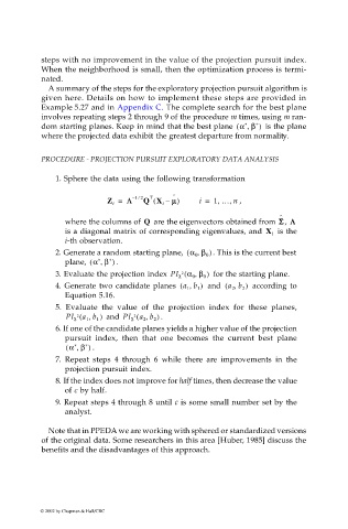
A summary of the steps for the exploratory projection pursuit algorithm is
given here. Details on how to implement these steps are provided in
Example 5.27 and in Appendix C. The complete search for the best plane
involves repeating steps 2 through 9 of the procedure m times, using m ran-
dom starting planes. Keep in mind that the best plane α β,( * * ) is the plane
where the projected data exhibit the greatest departure from normality.

PROCEDURE - PROJECTION PURSUIT EXPLORATORY DATA ANALYSIS

1. Sphere the data using the following transformation
ˆ
⁄
T
,
,
Z = Λ Λ Λ Λ – 12 Q X –( i µ µ µ µ) i = 1 … n ,
i
ˆ
Σ Σ Σ Σ
where the columns of Q are the eigenvectors obtained from , Λ ΛΛ Λ
is the
is a diagonal matrix of corresponding eigenvalues, and X i
i-th observation.
(
,
2. Generate a random starting plane, α 0 β 0 ) . This is the current best
plane, α β,( * * . )
3. Evaluate the projection index PI χ α 0 β 0 ) for the starting plane.
,
(
2
,
(
4. Generate two candidate planes a 1 b 1 ) and a 2 b 2 ) according to
(
,
Equation 5.16.
5. Evaluate the value of the projection index for these planes,
(
,
(
,
PI χ a 1 b 1 ) and PI χ a 2 b 2 ) .
2
2
6. If one of the candidate planes yields a higher value of the projection
pursuit index, then that one becomes the current best plane
( α β, * . )
*
7. Repeat steps 4 through 6 while there are improvements in the
projection pursuit index.
8. If the index does not improve for half times, then decrease the value
of c by half.
9. Repeat steps 4 through 8 until c is some small number set by the
analyst.
Note that in PPEDA we are working with sphered or standardized versions
of the original data. Some researchers in this area [Huber, 1985] discuss the
benefits and the disadvantages of this approach.

© 2002 by Chapman & Hall/CRC