Page 238 - Computational Statistics Handbook with MATLAB

Chapter 6: Monte Carlo Methods for Inferential Statistics 225

7. The lower endpoint of the interval is given by the bootstrap repli-
cate that is in the B α 2⁄⋅ -th position of the ordered θ ˆ *b , and the
upper endpoint is given by the bootstrap replicate that is in the
⁄
⋅
B ( 1 – α 2) -th position of the same ordered list. Alternatively,
using quantile notation, the lower endpoint is the estimated quan-
tile q ˆ α 2 and the upper endpoint is the estimated quantile q ˆ 1 – α 2 ,
⁄
⁄
where the estimates are taken from the bootstrap replicates.
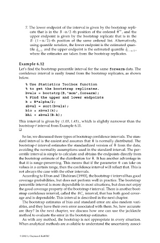
Example 6.12
Let’s find the bootstrap percentile interval for the same forearm data. The
confidence interval is easily found from the bootstrap replicates, as shown
below.
% Use Statistics Toolbox function
% to get the bootstrap replicates.
bvals = bootstrp(B,'mom',forearm);
% Find the upper and lower endpoints
k = B*alpha/2;
sbval = sort(bvals);
blo = sbval(k);
bhi = sbval(B-k);
This interval is given by 1.03 1.45,( ) , which is slightly narrower than the
bootstrap-t interval from Example 6.11.

So far, we discussed three types of bootstrap confidence intervals. The stan-
θ
ˆ
dard interval is the easiest and assumes that is normally distributed. The
θ
ˆ
bootstrap-t interval estimates the standardized version of from the data,
avoiding the normality assumptions used in the standard interval. The per-
centile interval is simple to calculate and obtains the endpoints directly from
ˆ
the bootstrap estimate of the distribution for θ. It has another advantage in
θ
that it is range-preserving. This means that if the parameter can take on
values in a certain range, then the confidence interval will reflect that. This is
not always the case with the other intervals.
According to Efron and Tibshirani [1993], the bootstrap-t interval has good
coverage probabilities, but does not perform well in practice. The bootstrap
percentile interval is more dependable in most situations, but does not enjoy
the good coverage property of the bootstrap-t interval. There is another boot-
interval, that has both good cover-
strap confidence interval, called the BC a
age and is dependable. This interval is described in the next chapter.
The bootstrap estimates of bias and standard error are also random vari-
ables, and they have their own error associated with them. So, how accurate
are they? In the next chapter, we discuss how one can use the jackknife
method to evaluate the error in the bootstrap estimates.
As with any method, the bootstrap is not appropriate in every situation.
When analytical methods are available to understand the uncertainty associ-

© 2002 by Chapman & Hall/CRC