Page 234 - Computational Statistics Handbook with MATLAB

Chapter 6: Monte Carlo Methods for Inferential Statistics 221

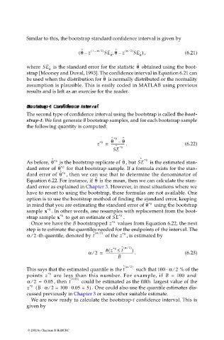
Similar to this, the bootstrap standard confidence interval is given by

ˆ
⁄
⁄
( θ – z ( 1 – α 2) SE ˆ θ –, ˆ z ( α 2) SE ˆ θ , ) (6.21)
θ
ˆ
θ
where SE ˆ θ is the standard error for the statistic obtained using the boot-
strap [Mooney and Duval, 1993]. The confidence interval in Equation 6.21 can
ˆ
θ
be used when the distribution for is normally distributed or the normality
assumption is plausible. This is easily coded in MATLAB using previous
results and is left as an exercise for the reader.
ddeencnc
ii
ee
IntervaInterva
l
Bootstrap-Bootstrap- Bootstrap- Bootstrap- t tt t ConfConfi ConfConf idde encnce eIntervaInterva l ll
The second type of confidence interval using the bootstrap is called the boot-
strap-t. We first generate B bootstrap samples, and for each bootstrap sample
the following quantity is computed:
ˆ *b ˆ
θ – θ
*b
z = ---------------- . (6.22)
ˆ *b
SE
As before, θ ˆ *b is the bootstrap replicate of , but SE is the estimated stan-
ˆ
θ
ˆ *b
dard error of θ ˆ *b for that bootstrap sample. If a formula exists for the stan-
dard error of θ ˆ *b , then we can use that to determine the denominator of
θ
ˆ
Equation 6.22. For instance, if is the mean, then we can calculate the stan-
dard error as explained in Chapter 3. However, in most situations where we
have to resort to using the bootstrap, these formulas are not available. One
option is to use the bootstrap method of finding the standard error, keeping
in mind that you are estimating the standard error of θ using the bootstrap
ˆ *b
sample x *b . In other words, one resamples with replacement from the boot-
ˆ *b
strap sample x *b to get an estimate of SE .
Once we have the B bootstrapped z *b values from Equation 6.22, the next
step is to estimate the quantiles needed for the endpoints of the interval. The
)
⁄
α 2 -th quantile, denoted by t ˆ α 2⁄( of the z *b , is estimated by
t
⁄
α 2 = # z ≤( *b ˆ α 2⁄( ) ) . (6.23)
---------------------------------
B
ˆ α 2⁄( )
This says that the estimated quantile is the t such that 100 α 2⁄⋅ % of the
points z *b are less than this number. For example, if B = 100 and
)
⁄
α 2 = 0.05 , then t ˆ 0.05( could be estimated as the fifth largest value of the
⋅
z *b B α 2⁄⋅( = 100 0.05 = 5) . One could also use the quantile estimates dis-
cussed previously in Chapter 3 or some other suitable estimate.
We are now ready to calculate the bootstrap-t confidence interval. This is
given by

© 2002 by Chapman & Hall/CRC