Page 229 - Computational Statistics Handbook with MATLAB

216 Computational Statistics Handbook with MATLAB

Efron and Tibshirani [1993] discuss a method called the parametric boot-
strap. In this case, the data analyst makes an assumption about the distribu-
tion that generated the original sample. Parameters for that distribution are
estimated from the sample, and resampling (in step 2) is done using the
assumed distribution and the estimated parameters. The parametric boot-
strap is closer to the Monte Carlo methods described in the previous section.
For instance, say we have reason to believe that the data come from an
λ
exponential distribution with parameter . We need to estimate the variance
and use

n
1
ˆ
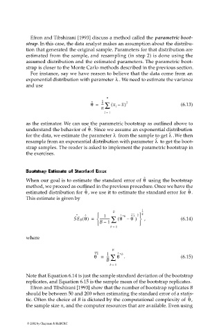
θ = --- ∑ ( x – x) 2 (6.13)
i
n
i = 1
as the estimator. We can use the parametric bootstrap as outlined above to
θ
ˆ
understand the behavior of . Since we assume an exponential distribution
λ
λ
ˆ
for the data, we estimate the parameter from the sample to get . We then
λ
ˆ
resample from an exponential distribution with parameter to get the boot-
strap samples. The reader is asked to implement the parametric bootstrap in
the exercises.
StandardErr
Bootstrap
Estimate
BootstrapEstimateof of Standard Er roor r
rr oorr
Standard
Estimate
StandardErEr
Bootstrap
BootstrapEstimateofof
ˆ
θ
When our goal is to estimate the standard error of using the bootstrap
method, we proceed as outlined in the previous procedure. Once we have the
estimated distribution for , we use it to estimate the standard error for . θ
θ
ˆ
ˆ
This estimate is given by
1 -- -
B
2
ˆ ˆ  1 ˆ *b ˆ *  2
SE B θ() =  ------------ ∑ ( θ – θ )  , (6.14)
 B – 1 
b = 1
where
B
ˆ
*
---
θ = 1 ∑ θ ˆ *b . (6.15)
B
b = 1
Note that Equation 6.14 is just the sample standard deviation of the bootstrap
replicates, and Equation 6.15 is the sample mean of the bootstrap replicates.
Efron and Tibshirani [1993] show that the number of bootstrap replicates B
should be between 50 and 200 when estimating the standard error of a statis-
ˆ
tic. Often the choice of B is dictated by the computational complexity of , θ
the sample size n, and the computer resources that are available. Even using
© 2002 by Chapman & Hall/CRC