Page 225 - Computational Statistics Handbook with MATLAB

212 Computational Statistics Handbook with MATLAB

M = 1000;
alpha = 0.05;
% Get the critical value, using z as test statistic.
cv = norminv(alpha,0,1);
% Start the simulation.
Im = 0;
for i = 1:M
% Generate a random sample under H_0.
xs = sigma*randn(1,n) + 454;
Tm = (mean(xs)-454)/sigxbar;
if Tm <= cv % then reject H_0
Im = Im +1;
end
end
alphahat = Im/M;
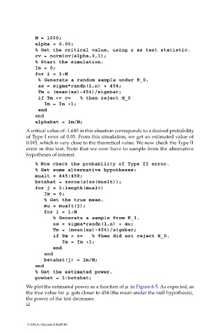
A critical value of -1.645 in this situation corresponds to a desired probability
of Type I error of 0.05. From this simulation, we get an estimated value of
0.045, which is very close to the theoretical value. We now check the Type II
error in this test. Note that we now have to sample from the alternative
hypotheses of interest.
% Now check the probability of Type II error.
% Get some alternative hypotheses:
mualt = 445:458;
betahat = zeros(size(mualt));
for j = 1:length(mualt)
Im = 0;
% Get the true mean.
mu = mualt(j);
for i = 1:M
% Generate a sample from H_1.
xs = sigma*randn(1,n) + mu;
Tm = (mean(xs)-454)/sigxbar;
if Tm > cv % Then did not reject H_0.
Im = Im +1;
end
end
betahat(j) = Im/M;
end
% Get the estimated power.
powhat = 1-betahat;
µ
We plot the estimated power as a function of in Figure 6.5. As expected, as
µ
the true value for gets closer to 454 (the mean under the null hypothesis),
the power of the test decreases.

© 2002 by Chapman & Hall/CRC