Page 221 - Computational Statistics Handbook with MATLAB

208 Computational Statistics Handbook with MATLAB

Normal Probability Plot
0.99
0.98
0.95
0.90

0.75
Probability 0.50

0.25

0.10
0.05
0.02
0.01
435 440 445 450 455 460 465
Data

G
I F F F F I I I URE GU 6. RE RE RE 6. 6. 6. 4 4
4
G
4
U
GU
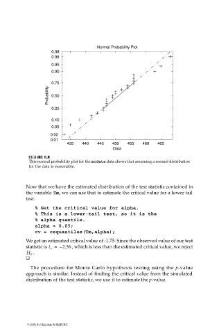
This normal probability plot for the mcdata data shows that assuming a normal distribution
for the data is reasonable.
Now that we have the estimated distribution of the test statistic contained in
the variable Tm, we can use that to estimate the critical value for a lower tail
test.
% Get the critical value for alpha.
% This is a lower-tail test, so it is the
% alpha quantile.
alpha = 0.05;
cv = csquantiles(Tm,alpha);
We get an estimated critical value of -1.75. Since the observed value of our test
statistic is t o = – 2.56 , which is less than the estimated critical value, we reject
.
H 0

The procedure for Monte Carlo hypothesis testing using the p-value
approach is similar. Instead of finding the critical value from the simulated
distribution of the test statistic, we use it to estimate the p-value.

© 2002 by Chapman & Hall/CRC