Page 226 - Computational Statistics Handbook with MATLAB

Chapter 6: Monte Carlo Methods for Inferential Statistics 213

1

0.9
0.8
0.7
Estimated Power 0.5
0.6

0.4
0.3
0.2
0.1
0
444 446 448 450 452 454 456 458
µ

IG
F FI U URE G 6. RE 6. 5 5
F F II GU RE RE 6. 6. 5
5
GU
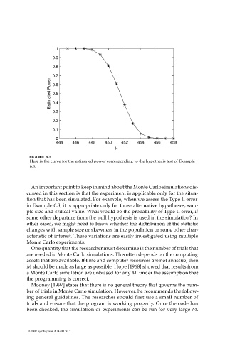
Here is the curve for the estimated power corresponding to the hypothesis test of Example
6.8.
An important point to keep in mind about the Monte Carlo simulations dis-
cussed in this section is that the experiment is applicable only for the situa-
tion that has been simulated. For example, when we assess the Type II error
in Example 6.8, it is appropriate only for those alternative hypotheses, sam-
ple size and critical value. What would be the probability of Type II error, if
some other departure from the null hypothesis is used in the simulation? In
other cases, we might need to know whether the distribution of the statistic
changes with sample size or skewness in the population or some other char-
acteristic of interest. These variations are easily investigated using multiple
Monte Carlo experiments.
One quantity that the researcher must determine is the number of trials that
are needed in Monte Carlo simulations. This often depends on the computing
assets that are available. If time and computer resources are not an issue, then
M should be made as large as possible. Hope [1968] showed that results from
a Monte Carlo simulation are unbiased for any M, under the assumption that
the programming is correct.
Mooney [1997] states that there is no general theory that governs the num-
ber of trials in Monte Carlo simulation. However, he recommends the follow-
ing general guidelines. The researcher should first use a small number of
trials and ensure that the program is working properly. Once the code has
been checked, the simulation or experiments can be run for very large M.

© 2002 by Chapman & Hall/CRC