Page 216 - Computational Statistics Handbook with MATLAB

Chapter 6: Monte Carlo Methods for Inferential Statistics 203

 ( α 2) X – µ ( 1 – α 2) 
⁄
⁄
Pz < --------------- < z  = 1 – α . (6.7)

σ ⁄
n
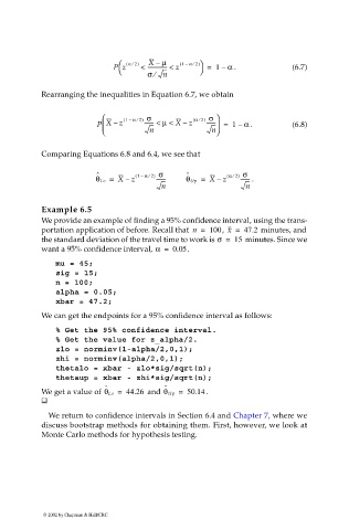
Rearranging the inequalities in Equation 6.7, we obtain
 ( α 2) σ ( α 2) σ 
⁄
⁄
P X – z 1 – ------- < µ < X – z -------  = 1 – α . (6.8)
 n n 
Comparing Equations 6.8 and 6.4, we see that

ˆ ( 1 – α 2) σ ˆ ( α 2) σ
⁄
⁄
θ Lo = X – z ------- θ Up = X – z ------- .
n n
Example 6.5
We provide an example of finding a 95% confidence interval, using the trans-
portation application of before. Recall that n = 100 , x = 47.2 minutes, and
the standard deviation of the travel time to work is σ = 15 minutes. Since we
want a 95% confidence interval, α = 0.05.
mu = 45;
sig = 15;
n = 100;
alpha = 0.05;
xbar = 47.2;
We can get the endpoints for a 95% confidence interval as follows:

% Get the 95% confidence interval.
% Get the value for z_alpha/2.
zlo = norminv(1-alpha/2,0,1);
zhi = norminv(alpha/2,0,1);
thetalo = xbar - zlo*sig/sqrt(n);
thetaup = xbar - zhi*sig/sqrt(n);
ˆ ˆ
We get a value of θ Lo = 44.26 and θ Up = 50.14 .

We return to confidence intervals in Section 6.4 and Chapter 7, where we
discuss bootstrap methods for obtaining them. First, however, we look at
Monte Carlo methods for hypothesis testing.

© 2002 by Chapman & Hall/CRC