Page 215 - Computational Statistics Handbook with MATLAB

202 Computational Statistics Handbook with MATLAB

⁄
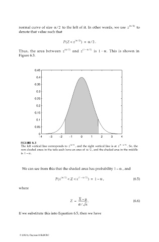
normal curve of size α 2⁄ to the left of it. In other words, we use z ( α 2) to
denote that value such that

⁄
PZ <( z ( α 2) ) = α . 2 ⁄
⁄
( α 2) ( 1 – α 2)
⁄
Thus, the area between z and z is 1 – α. This is shown in
Figure 6.3.

0.45
0.4

0.35
0.3

0.25
0.2
0.15

0.1
0.05

0
−4 −3 −2 −1 0 1 2 3 4

⁄
⁄
FI F F F U URE GU 6. RE RE RE 6. 6. 6. 3 3 ( α 2) ( 1 – α 2)
IG
GU
G
3
II
3
The left vertical line corresponds to z , and the right vertical line is at z . So, the
non-shaded areas in the tails each have an area of α 2⁄ , and the shaded area in the middle
is 1 – α .
We can see from this that the shaded area has probability 1 – α , and
⁄
⁄
Pz ( ( α 2) < Z < z ( 1 – α 2) ) = 1 – α , (6.5)
where
X – µ
Z = --------------- . (6.6)
σ ⁄ n

If we substitute this into Equation 6.5, then we have

© 2002 by Chapman & Hall/CRC