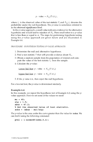
Page 213 - Computational Statistics Handbook with MATLAB

200 Computational Statistics Handbook with MATLAB

p – value = P ( T ≤ t , )
H 0 o
where is the observed value of the test statistic T, and P H .() denotes the
t o
0
probability under the null hypothesis. The p-value is sometimes referred to
as the observed significance level.
In the p-value approach, a small value indicates evidence for the alternative
. Here small refers to a p-value
hypothesis and would lead to rejection of H 0
that is less than or equal to α . The steps for performing hypothesis testing
using the p-value approach are given below and are illustrated in
Example 6.4.

PROCEDURE - HYPOTHESIS TESTING (P-VALUE APPROACH)

1. Determine the null and alternative hypotheses.
.
2. Find a test statistic T that will provide evidence about H 0
3. Obtain a random sample from the population of interest and com-
pute the value of the test statistic t o from the sample.
4. Calculate the p-value:

Lower Tail Test: p – value = P H T ≤( t o )
0
Upper Tail Test: p – value = P H T ≥( t o )
0
5. If the p-value ≤ α , then reject the null hypothesis.

For a two-tail test, the p-value is determined similarly.

Example 6.4
In this example, we repeat the hypothesis test of Example 6.2 using the p-
value approach. First we set some of the values we need:
mu = 45;
sig = 1.5;
xbar = 47.2;
% Get the observed value of test statistic.
zobs = (xbar - mu)/sig;
The p-value is the area under the curve greater than the value for zobs. We
can find it using the following command:
pval = 1-normcdf(zobs,0,1);

© 2002 by Chapman & Hall/CRC