Page 210 - Computational Statistics Handbook with MATLAB

Chapter 6: Monte Carlo Methods for Inferential Statistics 197

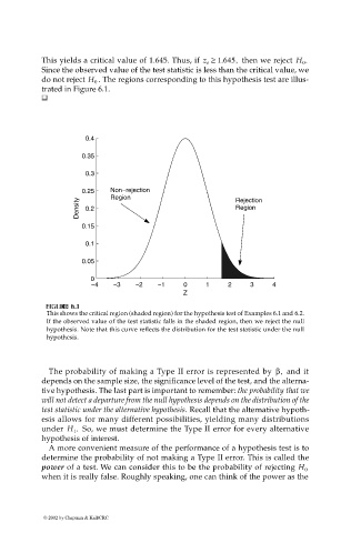
This yields a critical value of 1.645. Thus, if z o ≥ 1.645, then we reject H 0 .
Since the observed value of the test statistic is less than the critical value, we
. The regions corresponding to this hypothesis test are illus-
do not reject H 0
trated in Figure 6.1.

0.4

0.35

0.3
0.25 Non−rejection
Region Rejection
Density 0.2 Region

0.15

0.1
0.05

0
−4 −3 −2 −1 0 1 2 3 4
Z

IG
FI F U URE G 6. RE 6. 1 1
GU
1
F F II GU RE RE 6. 6. 1
This shows the critical region (shaded region) for the hypothesis test of Examples 6.1 and 6.2.
If the observed value of the test statistic falls in the shaded region, then we reject the null
hypothesis. Note that this curve reflects the distribution for the test statistic under the null
hypothesis.
The probability of making a Type II error is represented by β, and it
depends on the sample size, the significance level of the test, and the alterna-
tive hypothesis. The last part is important to remember: the probability that we
will not detect a departure from the null hypothesis depends on the distribution of the
test statistic under the alternative hypothesis. Recall that the alternative hypoth-
esis allows for many different possibilities, yielding many distributions
under H 1 . So, we must determine the Type II error for every alternative
hypothesis of interest.
A more convenient measure of the performance of a hypothesis test is to
determine the probability of not making a Type II error. This is called the
power of a test. We can consider this to be the probability of rejecting H 0
when it is really false. Roughly speaking, one can think of the power as the

© 2002 by Chapman & Hall/CRC