Page 321 - Computational Statistics Handbook with MATLAB

310 Computational Statistics Handbook with MATLAB

% Now generate 300 random variables. First find
% the number that fall in each one.
r = rand(1,n);
% Find the number generated from component 1.
ind = length(find(r <= pies(1)));
% Create some mixture data. Note that the
% component densities are normals.
x(1:ind) = randn(ind,1)*sqrt(vars(1)) + mus(1);
x(ind+1:n) = randn(n-ind,1)*sqrt(vars(2)) + mus(2);
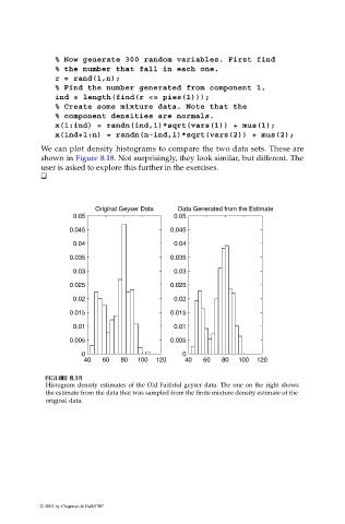
We can plot density histograms to compare the two data sets. These are
shown in Figure 8.18. Not surprisingly, they look similar, but different. The
user is asked to explore this further in the exercises.

Original Geyser Data Data Generated from the Estimate
0.05 0.05
0.045 0.045
0.04 0.04
0.035 0.035

0.03 0.03
0.025 0.025
0.02 0.02
0.015 0.015

0.01 0.01
0.005 0.005
0 0
40 60 80 100 120 40 60 80 100 120

U
GU
F FI F F II IG URE GU 8.1 RE RE RE 8.1 8 8 8 8
G
8.1
8.1
Histogram density estimates of the Old Faithful geyser data. The one on the right shows
the estimate from the data that was sampled from the finite mixture density estimate of the
original data.

© 2002 by Chapman & Hall/CRC