Page 316 - Computational Statistics Handbook with MATLAB

Chapter 8: Probability Density Estimation 305

(
,
(
,
,
(
;
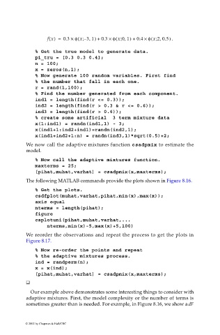
f x() = 0.3 × φ x 31) + 0.3 × φ x 01) + 0.4 × φ x 20.5 . )
;
;
–
% Get the true model to generate data.
pi_tru = [0.3 0.3 0.4];
n = 100;
x = zeros(n,1);
% Now generate 100 random variables. First find
% the number that fall in each one.
r = rand(1,100);
% Find the number generated from each component.
ind1 = length(find(r <= 0.3));
ind2 = length(find(r > 0.3 & r <= 0.6));
ind3 = length(find(r > 0.6));
% create some artificial 3 term mixture data
x(1:ind1) = randn(ind1,1) - 3;
x(ind1+1:ind2+ind1)=randn(ind2,1);
x(ind1+ind2+1:n) = randn(ind3,1)*sqrt(0.5)+2;
We now call the adaptive mixtures function csadpmix to estimate the
model.
% Now call the adaptive mixtures function.
maxterms = 25;
[pihat,muhat,varhat] = csadpmix(x,maxterms);
The following MATLAB commands provide the plots shown in Figure 8.16.

% Get the plots.
csdfplot(muhat,varhat,pihat,min(x),max(x));
axis equal
nterms = length(pihat);
figure
csplotuni(pihat,muhat,varhat,...
nterms,min(x)-5,max(x)+5,100)
We reorder the observations and repeat the process to get the plots in
Figure 8.17.

% Now re-order the points and repeat
% the adaptive mixtures process.
ind = randperm(n);
x = x(ind);
[pihat,muhat,varhat] = csadpmix(x,maxterms);

Our example above demonstrates some interesting things to consider with
adaptive mixtures. First, the model complexity or the number of terms is
sometimes greater than is needed. For example, in Figure 8.16, we show a dF

© 2002 by Chapman & Hall/CRC