Page 312 - Computational Statistics Handbook with MATLAB

Chapter 8: Probability Density Estimation 301

delpi = max(abs(mix_cof-mix_cofup));
deltol = max([delvar,delmu,delpi]);
% Reset parameters.
num_it = num_it+1;
mix_cof = mix_cofup;
mu = muup;
var_mat = varup;
end % while loop
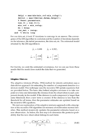
For our data set, it took 37 iterations to converge to an answer. The conver-
gence of the EM algorithm to a solution and the number of iterations depends
on the tolerance, the initial parameters, the data set, etc. The estimated model
returned by the EM algorithm is

ˆ
ˆ
p 1 = 0.498 p 2 = 0.502 ,

ˆ – 2.08 ˆ 1.83
µ 1 = µ 2 = .
2.03 – 0.03

For brevity, we omit the estimated covariances, but we can see from these
results that the model does match the data that we generated.

AdaptivAdaptiv
eMixtuMixtu
r
rees
Adaptiv
Adaptive ee MixtuMixtu rr eess s
The adaptive mixtures [Priebe, 1994] method for density estimation uses a
data-driven approach for estimating the number of component densities in a
mixture model. This technique uses the recursive EM update equations that
are provided below. The basic idea behind adaptive mixtures is to take one
point at a time and determine the distance from the observation to each com-
ponent density in the model. If the distance to each component is larger than
some threshold, then a new term is created. If the distance is less than the
threshold for all terms, then the parameter estimates are updated based on
the recursive EM equations.
We start our explanation of the adaptive mixtures approach with a descrip-
tion of the recursive EM algorithm for mixtures of multivariate normal den-
sities. This method recursively updates the parameter estimates based on a
new observation. As before, the first step is to determine the posterior prob-
ability that the new observation belongs to each term:

n ()
Σ i )
µ i ,
ˆ
;
ˆ n +( 1) p i φ x( ( n + 1) ˆ n() ˆ n() 1 …,
,
τ i = -----------------------------------------------------; i = , c (8.40)
ˆ n() ( n + 1)
f ( x )
© 2002 by Chapman & Hall/CRC