Page 309 - Computational Statistics Handbook with MATLAB

298 Computational Statistics Handbook with MATLAB

ˆ
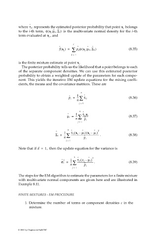
where τ ij represents the estimated posterior probability that point belongs
x j
ˆ ˆ
,
to the i-th term, φ x j µ i Σ i) is the multivariate normal density for the i-th
(
;
, and
term evaluated at x j
c
ˆ ˆ ˆ ˆ
,
(
f x () = ∑ p φ x µ k Σ k) (8.35)
;
j
k
j
k = 1
is the finite mixture estimate at point x j .
The posterior probability tells us the likelihood that a point belongs to each
of the separate component densities. We can use this estimated posterior
probability to obtain a weighted update of the parameters for each compo-
nent. This yields the iterative EM update equations for the mixing coeffi-
cients, the means and the covariance matrices. These are
n
ˆ
p i = 1 ∑ ˆ τ ij (8.36)
---
n
j = 1
n
ˆ
ˆ 1 τ ijx j
µ i = --- ∑ --------- (8.37)
ˆ
n p i
j = 1
n T
ˆ
ˆ
ˆ
ˆ 1 τ ij x j –( µ i) x j –( µ i)
Σ i = --- ∑ ------------------------------------------------ . (8.38)
n ˆ p i
j = 1
Note that if d = 1, then the update equation for the variance is
n ˆ ˆ 2
ˆ 2 1 τ ij x j –( µ i)
σ i = --- ∑ --------------------------- . (8.39)
ˆ
n p i
j = 1
The steps for the EM algorithm to estimate the parameters for a finite mixture
with multivariate normal components are given here and are illustrated in
Example 8.11.

FINITE MIXTURES - EM PROCEDURE
1. Determine the number of terms or component densities c in the
mixture.

© 2002 by Chapman & Hall/CRC