Page 306 - Computational Statistics Handbook with MATLAB

Chapter 8: Probability Density Estimation 295

% corresponds to a d-D mean; a 3-D array of
% covariances, where each page of the array is a
% covariance matrix.
pies = [0.5 0.3 0.2]; % mixing coefficients
mus = [-1 1 5; -1 1 6];
% Delete any previous variances in the workspace.
clear vars
vars(:,:,1) = eye(2);
vars(:,:,2) = eye(2)*.5
vars(:,:,3) = [1 0.5; 0.5 1];
figure
csdfplot(mus,vars,pies)
The resulting plot is shown in Figure 8.14. Note that the covariance of two of
the component densities are represented by circles, with one larger than the
other. These correspond to the first two terms of the model. The third compo-
nent density has an elliptical covariance structure indicating non-zero off-
diagonal elements in the covariance matrix. We now do the same thing for the
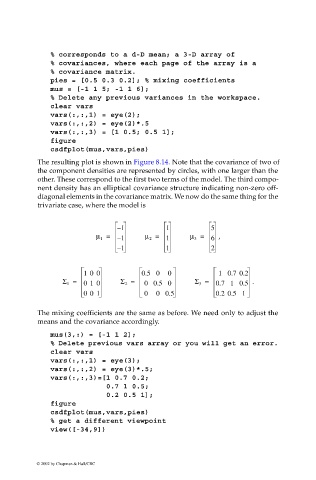
trivariate case, where the model is

– 1 1 5
µ 1 = – 1 µ 2 = 1 µ 3 = 6 ,

– 1 1 2

10 0 0.5 0 0 10.7 0.2
Σ 1 = 01 0 Σ 2 = 00.50 Σ 3 = 0.710.5 .
00 1 0 0 0.5 0.2 0.5 1

The mixing coefficients are the same as before. We need only to adjust the
means and the covariance accordingly.

mus(3,:) = [-1 1 2];
% Delete previous vars array or you will get an error.
clear vars
vars(:,:,1) = eye(3);
vars(:,:,2) = eye(3)*.5;
vars(:,:,3)=[1 0.7 0.2;
0.7 1 0.5;
0.2 0.5 1];
figure
csdfplot(mus,vars,pies)
% get a different viewpoint
view([-34,9])

© 2002 by Chapman & Hall/CRC