Page 302 - Computational Statistics Handbook with MATLAB

Chapter 8: Probability Density Estimation 291

3 Term Finite Mixture
0.35

0.3

0.25

0.2

0.15

0.1

0.05

0
−6 −4 −2 0 2 4 6
x

II
IG
F F FI F U URE G 8.12 RE RE RE 8.12
GU
8.12
8.12
GU
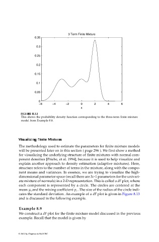
This shows the probability density function corresponding to the three-term finite mixture
model from Example 8.8.
isu
Visu
nngFiniFini
g
al
VVisuisu
r
V a aall li ii izzi zzii inngFinigFinit teeMixtuMixtu rr eess s
rees
ee
tt
MixtuMixtu
The methodology used to estimate the parameters for finite mixture models
will be presented later on in this section ( page 296 ). We first show a method
for visualizing the underlying structure of finite mixtures with normal com-
ponent densities [Priebe, et al. 1994], because it is used to help visualize and
explain another approach to density estimation (adaptive mixtures). Here,
structure refers to the number of terms in the mixture, along with the compo-
nent means and variances. In essence, we are trying to visualize the high-
dimensional parameter space (recall there are 3c-1 parameters for the univari-
ate mixture of normals) in a 2-D representation. This is called a dF plot, where
each component is represented by a circle. The circles are centered at the
and the mixing coefficient . The size of the radius of the circle indi-
mean µ i p i
cates the standard deviation. An example of a dF plot is given in Figure 8.13
and is discussed in the following example.
Example 8.9
We construct a dF plot for the finite mixture model discussed in the previous
example. Recall that the model is given by

© 2002 by Chapman & Hall/CRC