Page 297 - Computational Statistics Handbook with MATLAB

286 Computational Statistics Handbook with MATLAB

width in each dimension. Since the product kernel estimate is comprised of
univariate kernels, we can use any of the kernels that were discussed previ-
ously.
Scott [1992] gives expressions for the asymptotic integrated squared bias
and asymptotic integrated variance for the multivariate product kernel. If the
normal kernel is used, then minimizing these yields a normal reference rule
for the multivariate case, which is given below.

NORMAL REFERENCE RULE - KERNEL (MULTIVARIATE)

1
------------
4
*  -------------------- d + 4 1 …,
,
(
h j =  nd + 2) σ j ; j = , d
Ker
can be used. If there is any skewness or kur-
where a suitable estimate for σ j
tosis evident in the data, then the window widths should be narrower, as dis-
cussed previously. The skewness factor for the frequency polygon
(Equation 8.20) can be used here.
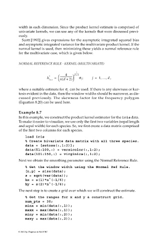
Example 8.7
In this example, we construct the product kernel estimator for the iris data.
To make it easier to visualize, we use only the first two variables (sepal length
and sepal width) for each species. So, we first create a data matrix comprised
of the first two columns for each species.
load iris
% Create bivariate data matrix with all three species.
data = [setosa(:,1:2)];
data(51:100,:) = versicolor(:,1:2);
data(101:150,:) = virginica(:,1:2);
Next we obtain the smoothing parameter using the Normal Reference Rule.

% Get the window width using the Normal Ref Rule.
[n,p] = size(data);
s = sqrt(var(data));
hx = s(1)*n^(-1/6);
hy = s(2)*n^(-1/6);
The next step is to create a grid over which we will construct the estimate.
% Get the ranges for x and y & construct grid.
num_pts = 30;
minx = min(data(:,1));
maxx = max(data(:,1));
miny = min(data(:,2));
maxy = max(data(:,2));

© 2002 by Chapman & Hall/CRC