Page 294 - Computational Statistics Handbook with MATLAB

Chapter 8: Probability Density Estimation 283

h = 0.84 h = 0.42
0.8 0.8

0.6 0.6
0.4 0.4
0.2 0.2

0 0
−4 −2 0 2 4 −4 −2 0 2 4
h = 0.21 h = 0.11
0.8 0.8

0.6 0.6
0.4 0.4
0.2 0.2
0 0
−4 −2 0 2 4 −4 −2 0 2 4

U
FI F IG URE G 8.9 RE 8.9
8.9
F F II GU RE RE 8.9
GU
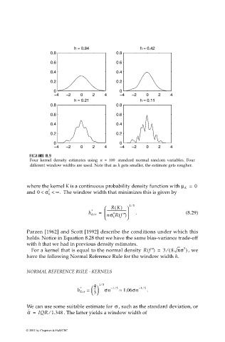
Four kernel density estimates using n = 100 standard normal random variables. Four
different window widths are used. Note that as h gets smaller, the estimate gets rougher.
where the kernel K is a continuous probability density function with µ K = 0
and 0 < σ K < ∞. The window width that minimizes this is given by
2

⁄
 RK()  15
* -----------------------
h Ker =  nσ Rf ″()  . (8.29)
4
 k 
Parzen [1962] and Scott [1992] describe the conditions under which this
holds. Notice in Equation 8.28 that we have the same bias-variance trade-off
with h that we had in previous density estimates.
5
For a kernel that is equal to the normal density Rf ″() = 3 (⁄ 8 πσ ) , we
have the following Normal Reference Rule for the window width h.

NORMAL REFERENCE RULE - KERNELS

⁄
4 15
⁄
⁄
* --  – 15 – 15
-
h Ker = 3  σn ≈ 1.06σn .
σ
We can use some suitable estimate for , such as the standard deviation, or
⁄
ˆ
σ = IQR 1.348 . The latter yields a window width of
© 2002 by Chapman & Hall/CRC