Page 295 - Computational Statistics Handbook with MATLAB

284 Computational Statistics Handbook with MATLAB

⁄
ˆ * – 15
h Ker = 0.786 × IQR × n .
Silverman [1986] recommends that one use whichever is smaller, the sample
standard deviation or IQR 1.348⁄ as an estimate for . σ
We now turn our attention to the problem of what kernel to use in our esti-
mate. It is known [Scott, 1992] that the choice of smoothing parameter h is
more important than choosing the kernel. This arises from the fact that the
effects from the choice of kernel (e.g., kernel tail behavior) are reduced by the
averaging process. We discuss the efficiency of the kernels below, but what
really drives the choice of a kernel are computational considerations or the
amount of differentiability required in the estimate.
In terms of efficiency, the optimal kernel was shown to be [Epanechnikov,
1969]

 3
 -- 1 –( t ); – 1 ≤≤ 1
2
t
-
Kt() =  4

 0; otherwise.
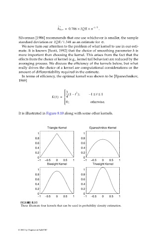
It is illustrated in Figure 8.10 along with some other kernels.

Triangle Kernel Epanechnikov Kernel
1 1
0.8 0.8
0.6 0.6
0.4 0.4
0.2 0.2
0 0
−1 −0.5 0 0.5 1 −1 −0.5 0 0.5 1
Biweight Kernel Triweight Kernel
1 1
0.8 0.8
0.6 0.6
0.4 0.4
0.2 0.2
0 0
−1 −0.5 0 0.5 1 −1 −0.5 0 0.5 1
II
U
F F FI F IG URE G 8.10 RE RE RE 8.10
GU
8.10
8.10
GU
These illustrate four kernels that can be used in probability density estimation.
© 2002 by Chapman & Hall/CRC