Page 293 - Computational Statistics Handbook with MATLAB

282 Computational Statistics Handbook with MATLAB

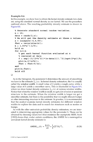
Example 8.6
In this example, we show how to obtain the kernel density estimate for a data
set, using the standard normal density as our kernel. We use the procedure
outlined above. The resulting probability density estimate is shown in
Figure 8.8.
% Generate standard normal random variables.
n = 10;
data = randn(1,n);
% We will get the density estimate at these x values.
x = linspace(-4,4,50);
fhat = zeros(size(x));
h = 1.06*n^(-1/5);
hold on
for i=1:n
% get each kernel function evaluated at x
% centered at data
f = exp(-(1/(2*h^2))*(x-data(i)).^2)/sqrt(2*pi)/h;
plot(x,f/(n*h));
fhat = fhat+f/(n);
end
plot(x,fhat);
hold off

As in the histogram, the parameter h determines the amount of smoothing
ˆ
we have in the estimate f Ker x() . In kernel density estimation, the h is usually
called the window width. A small value of h yields a rough curve, while a
large value of h yields a smoother curve. This is illustrated in Figure 8.9,
ˆ
where we show kernel density estimates f Ker x() at various window widths.
Notice that when the window width is small, we get a lot of noise or spurious
structure in the estimate. When the window width is larger we get a
smoother estimate, but there is the possibility that we might obscure bumps
or other interesting structure in the estimate. In practice, it is recommended
that the analyst examine kernel density estimates for different window
widths to explore the data and to search for structures such as modes or
bumps.
As with the other univariate probability density estimators, we are inter-
ested in determining appropriate values for the parameter h. These can be
obtained by choosing values for h that minimize the asymptotic MISE. Scott
[1992] shows that, under certain conditions, the AMISE for a nonnegative
univariate kernel density estimator is

RK() 1 4 4
-
AMISE Ker h() = ------------- + --σ k h Rf ″() , (8.28)
nh 4

© 2002 by Chapman & Hall/CRC