Page 289 - Computational Statistics Handbook with MATLAB

278 Computational Statistics Handbook with MATLAB

Example 8.5
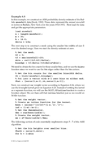
In this example, we construct an ASH probability density estimate of the Buf-
falo snowfall data [Scott, 1992]. These data represent the annual snowfall
in inches in Buffalo, New York over the years 1910-1972. First load the data
and get the appropriate parameters.
load snowfall
n = length(snowfall);
m = 30;
h = 14.6;
delta = h/m;
The next step is to construct a mesh using the smaller bin widths of size δ
over the desired range. Here we start the density estimate at zero.
% Get the mesh.
t0 = 0;
tf = max(snowfall)+20;
nbin = ceil((tf-t0)/delta);
binedge = t0:delta:(t0+delta*nbin);

We need to obtain the bin counts for these smaller bins, and we use the histc
function since we want to use the bin edges rather than the bin centers.
% Get the bin counts for the smaller binwidth delta.
vk = histc(snowfall,binedge);
% Put into a vector with m-1 zero bins on either end.
fhat = [zeros(1,m-1),vk,zeros(1,m-1)];
Next, we construct our weight vector according to Equation 8.24, where we
use the biweight kernel given in Equation 8.25. Instead of writing the kernel
as a separate function, we will use the MATLAB inline function to create a
function object. We can then call that inline function just as we would an
M-file function.
% Get the weight vector.
% Create an inline function for the kernel.
kern = inline('(15/16)*(1-x.^2).^2');
ind = (1-m):(m-1);
% Get the denominator.
den = sum(kern(ind/m));
% Create the weight vector.
wm = m*(kern(ind/m))/den;
The following section of code essentially implements steps 5 - 7 of the ASH
algorithm.

% Get the bin heights over smaller bins.
fhatk = zeros(1,nbin);
for k = 1:nbin

© 2002 by Chapman & Hall/CRC