Page 285 - Computational Statistics Handbook with MATLAB

274 Computational Statistics Handbook with MATLAB

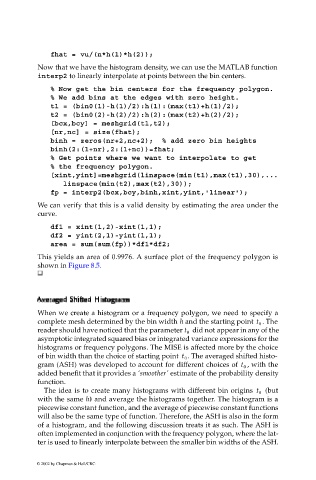
fhat = vu/(n*h(1)*h(2));
Now that we have the histogram density, we can use the MATLAB function
interp2 to linearly interpolate at points between the bin centers.

% Now get the bin centers for the frequency polygon.
% We add bins at the edges with zero height.
t1 = (bin0(1)-h(1)/2):h(1):(max(t1)+h(1)/2);
t2 = (bin0(2)-h(2)/2):h(2):(max(t2)+h(2)/2);
[bcx,bcy] = meshgrid(t1,t2);
[nr,nc] = size(fhat);
binh = zeros(nr+2,nc+2); % add zero bin heights
binh(2:(1+nr),2:(1+nc))=fhat;
% Get points where we want to interpolate to get
% the frequency polygon.
[xint,yint]=meshgrid(linspace(min(t1),max(t1),30),...
linspace(min(t2),max(t2),30));
fp = interp2(bcx,bcy,binh,xint,yint,'linear');
We can verify that this is a valid density by estimating the area under the
curve.

df1 = xint(1,2)-xint(1,1);
df2 = yint(2,1)-yint(1,1);
area = sum(sum(fp))*df1*df2;
This yields an area of 0.9976. A surface plot of the frequency polygon is
shown in Figure 8.5.

Av
Ave
ged
AvAv er eerr aagedShiftedHistogramHistogram ss s
Shifted
s
ged
Shifted
raagedShiftedHistogramHistogram
When we create a histogram or a frequency polygon, we need to specify a
complete mesh determined by the bin width h and the starting point . The
t 0
reader should have noticed that the parameter did not appear in any of the
t 0
asymptotic integrated squared bias or integrated variance expressions for the
histograms or frequency polygons. The MISE is affected more by the choice
of bin width than the choice of starting point . The averaged shifted histo-
t 0
, with the
gram (ASH) was developed to account for different choices of t 0
added benefit that it provides a ‘smoother’ estimate of the probability density
function.
(but
The idea is to create many histograms with different bin origins t 0
with the same h) and average the histograms together. The histogram is a
piecewise constant function, and the average of piecewise constant functions
will also be the same type of function. Therefore, the ASH is also in the form
of a histogram, and the following discussion treats it as such. The ASH is
often implemented in conjunction with the frequency polygon, where the lat-
ter is used to linearly interpolate between the smaller bin widths of the ASH.
© 2002 by Chapman & Hall/CRC