Page 284 - Computational Statistics Handbook with MATLAB

Chapter 8: Probability Density Estimation 273

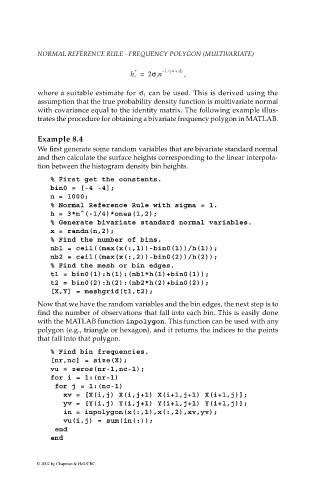
NORMAL REFERENCE RULE - FREQUENCY POLYGON (MULTIVARIATE)

⁄
*
h i = 2σ i n – 1 ( 4 + d) ,
can be used. This is derived using the
where a suitable estimate for σ i
assumption that the true probability density function is multivariate normal
with covariance equal to the identity matrix. The following example illus-
trates the procedure for obtaining a bivariate frequency polygon in MATLAB.

Example 8.4
We first generate some random variables that are bivariate standard normal
and then calculate the surface heights corresponding to the linear interpola-
tion between the histogram density bin heights.

% First get the constants.
bin0 = [-4 -4];
n = 1000;
% Normal Reference Rule with sigma = 1.
h = 3*n^(-1/4)*ones(1,2);
% Generate bivariate standard normal variables.
x = randn(n,2);
% Find the number of bins.
nb1 = ceil((max(x(:,1))-bin0(1))/h(1));
nb2 = ceil((max(x(:,2))-bin0(2))/h(2));
% Find the mesh or bin edges.
t1 = bin0(1):h(1):(nb1*h(1)+bin0(1));
t2 = bin0(2):h(2):(nb2*h(2)+bin0(2));
[X,Y] = meshgrid(t1,t2);
Now that we have the random variables and the bin edges, the next step is to
find the number of observations that fall into each bin. This is easily done
with the MATLAB function inpolygon. This function can be used with any
polygon (e.g., triangle or hexagon), and it returns the indices to the points
that fall into that polygon.

% Find bin frequencies.
[nr,nc] = size(X);
vu = zeros(nr-1,nc-1);
for i = 1:(nr-1)
for j = 1:(nc-1)
xv = [X(i,j) X(i,j+1) X(i+1,j+1) X(i+1,j)];
yv = [Y(i,j) Y(i,j+1) Y(i+1,j+1) Y(i+1,j)];
in = inpolygon(x(:,1),x(:,2),xv,yv);
vu(i,j) = sum(in(:));
end
end

© 2002 by Chapman & Hall/CRC