Page 279 - Computational Statistics Handbook with MATLAB

268 Computational Statistics Handbook with MATLAB

,
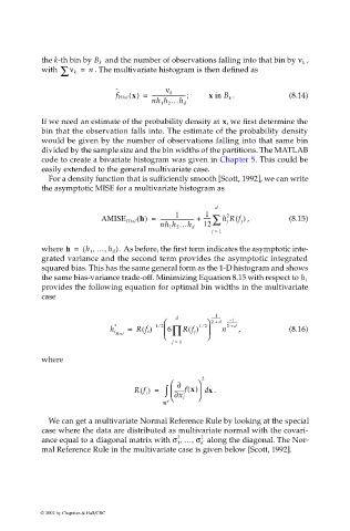
the k-th bin by B k and the number of observations falling into that bin by ν k
with ∑ ν k = n . The multivariate histogram is then defined as

ˆ ν k
f Hist x() = --------------------------; x in B k . (8.14)
nh 1 h 2 …h d
If we need an estimate of the probability density at x, we first determine the
bin that the observation falls into. The estimate of the probability density
would be given by the number of observations falling into that same bin
divided by the sample size and the bin widths of the partitions. The MATLAB
code to create a bivariate histogram was given in Chapter 5. This could be
easily extended to the general multivariate case.
For a density function that is sufficiently smooth [Scott, 1992], we can write
the asymptotic MISE for a multivariate histogram as

d
1 1 2
AMISE Hist h () = -------------------------- + ----- - ∑ h Rf () , (8.15)
j
j
nh 1 h 2 …h d 12
j = 1
,
,
where h = ( h 1 … h d ). As before, the first term indicates the asymptotic inte-
grated variance and the second term provides the asymptotic integrated
squared bias. This has the same general form as the 1-D histogram and shows
the same bias-variance trade-off. Minimizing Equation 8.15 with respect to h i
provides the following equation for optimal bin widths in the multivariate
case

1
------------
d
1
  2 + d ------------
–
⁄
⁄
* Rf i () – 12 6  Rf j () 12 2 + d
h i = ∏  n , (8.16)
 
Hist
j = 1
where
2
 ∂ 

Rf () = ∫   ∂ x i f x() d . x
i

ℜ d
We can get a multivariate Normal Reference Rule by looking at the special
case where the data are distributed as multivariate normal with the covari-
ance equal to a diagonal matrix with σ …σ, , 2 d along the diagonal. The Nor-
2
1
mal Reference Rule in the multivariate case is given below [Scott, 1992].

© 2002 by Chapman & Hall/CRC