Page 281 - Computational Statistics Handbook with MATLAB

270 Computational Statistics Handbook with MATLAB

0.25

0.2

0.15

0.1

0.05

0
B B
k k+1
IG
FI F U URE G 8. RE 8. 3 3
GU
3
F F II GU RE RE 8. 8. 3
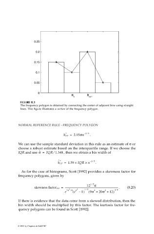
The frequency polygon is obtained by connecting the center of adjacent bins using straight
lines. This figure illustrates a section of the frequency polygon.
NORMAL REFERENCE RULE - FREQUENCY POLYGON

⁄
*
h FP = 2.15σn – 15 .
We can use the sample standard deviation in this rule as an estimate of σ or
choose a robust estimate based on the interquartile range. If we choose the
ˆ
⁄
IQR and use σ = IQR 1.348 , then we obtain a bin width of
⁄
ˆ * – 15
h FP = 1.59 × IQR × n .
As for the case of histograms, Scott [1992] provides a skewness factor for
frequency polygons, given by

⁄
12 15 σ
skewness factor FP = ------------------------------------------------------------------------------------------- . (8.20)
⁄
2
⁄
7σ ⁄ 4 σ 2 12 4 2 15
e ( e – 1) ( 9σ + 20σ + 12)
If there is evidence that the data come from a skewed distribution, then the
bin width should be multiplied by this factor. The kurtosis factor for fre-
quency polygons can be found in Scott [1992].

© 2002 by Chapman & Hall/CRC