Page 286 - Computational Statistics Handbook with MATLAB

Chapter 8: Probability Density Estimation 275

0.1

0.05

0
2
0 2
0
−2
−2
−4 −4
II
IG
GU
GU
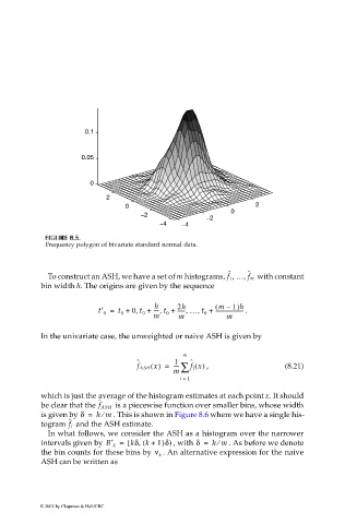
F F FI F U URE G 8.5. RE RE RE 8.5. 8.5. 8.5.
Frequency polygon of bivariate standard normal data.
ˆ , , ˆ
To construct an ASH, we have a set of m histograms, f 1 … f m with constant
bin width h. The origins are given by the sequence
h
m –
1)h
------ … t +,
,
t′ = t + 0 t +, 0 ---- t + 2h , 0 ( --------------------- .
0
0
0
m m m
In the univariate case, the unweighted or naive ASH is given by
m
ˆ 1 ˆ
f ASH x() = ---- ∑ f i x() , (8.21)
m
i = 1
which is just the average of the histogram estimates at each point x. It should
ˆ
be clear that the f ASH is a piecewise function over smaller bins, whose width
⁄
is given by δ = hm . This is shown in Figure 8.6 where we have a single his-
ˆ
togram and the ASH estimate.
f i
In what follows, we consider the ASH as a histogram over the narrower
⁄
,
(
intervals given by B′ = [kδ k + 1)δ) , with δ = hm . As before we denote
k
the bin counts for these bins by ν k . An alternative expression for the naive
ASH can be written as
© 2002 by Chapman & Hall/CRC