Page 287 - Computational Statistics Handbook with MATLAB

276 Computational Statistics Handbook with MATLAB

Histogram Density ASH − m=5
0.5 0.5

0.45 0.45
0.4 0.4
0.35 0.35
0.3 0.3
0.25 0.25

0.2 0.2
0.15 0.15
0.1 0.1
0.05 0.05
0 0
−4 −2 0 2 4 −4 −2 0 2 4

F FI U URE G 8.6 RE 8.6
IG
F F II GU RE RE 8.6
GU
8.6
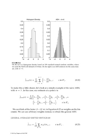
On the left is a histogram density based on 100 standard normal random variables, where
we used the MATLAB default of 10 bins. On the right is an ASH estimate for the same data
set, with m = 5.
m – 1
ˆ 1  i 
f ASH x() = ------ ∑  1 – ---- ν k + ; x in B′ k . (8.22)

i
nh m
i = 1 – m
To make this a little clearer, let’s look at a simple example of the naive ASH,
with m = 3 . In this case, our estimate at a point x is

ˆ 1  2   1  0
-
-
f ASH x() = ------ 1 – -- ν k – + 1 – -- ν k – + 1 – -- ν k – +
-
nh  3  2  3  1  3  0
 1   2
-
-


 1 – -- ν k + +  1 – -- ν k + 2 ; x in B′ k .
1
3
3
⁄
We can think of the factor 1 –( im) in Equation 8.22 as weights on the bin
counts. We can use arbitrary weights instead, to obtain the general ASH.
GENERAL AVERAGED SHIFTED HISTOGRAM
ˆ 1
f ASH = ------ ∑ w m i()ν k + ; x in B′ k . (8.23)
i
nh
i < m
© 2002 by Chapman & Hall/CRC