Page 290 - Computational Statistics Handbook with MATLAB

Chapter 8: Probability Density Estimation 279

ind = k:(2*m+k-2);
fhatk(k) = sum(wm.*fhat(ind));
end
fhatk = fhatk/(n*h);
bc = t0+((1:k)-0.5)*delta;
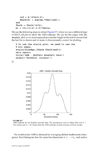
We use the following steps to obtain Figure 8.7, where we use a different type
of MATLAB plot to show the ASH estimate. We use the bin edges with the
stairs plot, so we must append an extra bin height at the end to ensure that
the last bin is drawn and to make it dimensionally correct for plotting.
% To use the stairs plot, we need to use the
% bin edges.
stairs(binedge,[fhatk fhatk(end)])
axis square
title('ASH - Buffalo Snowfall Data')
xlabel('Snowfall (inches)')

ASH − Buffalo Snowfall Data
0.02
0.018
0.016
0.014

0.012
0.01
0.008
0.006

0.004
0.002
0
0 50 100 150
Snowfall (inches)

F FI U URE G 8.7 RE 8.7
IG
F F II GU RE RE 8.7
GU
8.7
ASH estimate for the Buffalo snowfall data. The parameters used to obtain this were h =
14.6 inches and m = 30. Notice that the ASH estimate reveals evidence of three modes.
The multivariate ASH is obtained by averaging shifted multivariate histo-
grams. Each histogram has the same bin dimension h 1 × … × h d , and each is

© 2002 by Chapman & Hall/CRC