Page 288 - Computational Statistics Handbook with MATLAB

Chapter 8: Probability Density Estimation 277

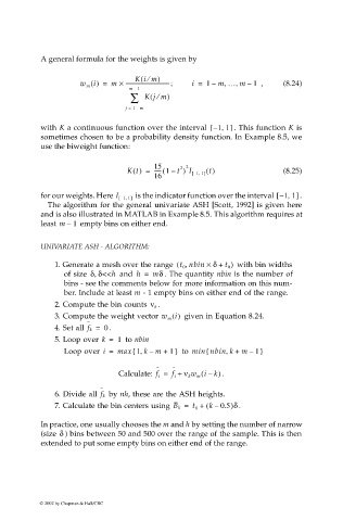
A general formula for the weights is given by

⁄
(
Ki m)
,
,
w m i() = m × ----------------------------------; i = 1 – m … m – 1 , (8.24)
m – 1
∑ Kj m)
⁄
(
j = 1 – m
,
with K a continuous function over the interval –[ 1 1] . This function K is
sometimes chosen to be a probability density function. In Example 8.5, we
use the biweight function:
15 2 2
-
Kt() = ----- 1 –( t ) I –[ 1 1] t() (8.25)
,
16
,
is the indicator function over the interval –[ 1 1]
,
for our weights. Here I –[ 1 1] .
The algorithm for the general univariate ASH [Scott, 1992] is given here
and is also illustrated in MATLAB in Example 8.5. This algorithm requires at
least m – 1 empty bins on either end.
UNIVARIATE ASH - ALGORITHM:

1. Generate a mesh over the range t 0 nbin ×,( δ + ) with bin widths
t 0
of size δδ<<h, and h = mδ . The quantity nbin is the number of
bins - see the comments below for more information on this num-
ber. Include at least m - 1 empty bins on either end of the range.
.
2. Compute the bin counts ν k
3. Compute the weight vector w m i() given in Equation 8.24.
ˆ
4. Set all f k = . 0
5. Loop over k = 1 to nbin
{
,
Loop over i = max 1 k – m + 1} to min nbin k +,{ m – 1}
ˆ ˆ
Calculate: f i = f i + ν k w m i –( k) .
ˆ
6. Divide all by nh, these are the ASH heights.
f k
7. Calculate the bin centers using B k = t 0 + ( k – 0.5)δ .
In practice, one usually chooses the m and h by setting the number of narrow
δ
(size ) bins between 50 and 500 over the range of the sample. This is then
extended to put some empty bins on either end of the range.

© 2002 by Chapman & Hall/CRC