Page 280 - Computational Statistics Handbook with MATLAB

Chapter 8: Probability Density Estimation 269

NORMAL REFERENCE RULE - MULTIVARIATE HISTOGRAMS

– 1
------------
,
* ≈ 2 + d 1 …,
h i 3.5σ i n ; i = . d
Hist
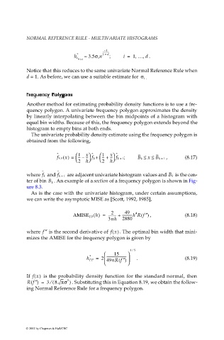
Notice that this reduces to the same univariate Normal Reference Rule when
d = 1. As before, we can use a suitable estimate for σ i .

c
cyPolygonsyPolygons
y
Freequenquen
Fr
FFrr eequenquen ccyPolygonsPolygons
Another method for estimating probability density functions is to use a fre-
quency polygon. A univariate frequency polygon approximates the density
by linearly interpolating between the bin midpoints of a histogram with
equal bin widths. Because of this, the frequency polygon extends beyond the
histogram to empty bins at both ends.
The univariate probability density estimate using the frequency polygon is
obtained from the following,
ˆ 1  x ˆ 1  x ˆ
f FP x() = -- – --- f k + -- + -- f k + ; B k ≤ x ≤ , (8.17)
-
-
-
 2 h   2 h  1 B k + 1
ˆ ˆ
f k
where and f k + 1 are adjacent univariate histogram values and B k is the cen-
. An example of a section of a frequency polygon is shown in Fig-
ter of bin B k
ure 8.3.
As is the case with the univariate histogram, under certain assumptions,
we can write the asymptotic MISE as [Scott, 1992, 1985],
2 -----------h Rf ″()
49
4
h
AMISE () = ---------- + - , (8.18)
FP
3nh 2880
where f ″ is the second derivative of f x() . The optimal bin width that mini-
mizes the AMISE for the frequency polygon is given by
⁄
15
 15 
* -----------------------
h FP = 2 49nR f ″()  . (8.19)
 
If f x() is the probability density function for the standard normal, then
5
Rf ″() = 3 (⁄ 8 πσ ) . Substituting this in Equation 8.19, we obtain the follow-
ing Normal Reference Rule for a frequency polygon.

© 2002 by Chapman & Hall/CRC