Page 276 - Computational Statistics Handbook with MATLAB

Chapter 8: Probability Density Estimation 265

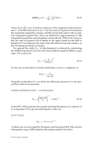
1
1 ------h Rf()
2
AMISE Hist h() = ------ + , ′ (8.10)
nh 12
2
where Rg() ≡ ∫ g x() xd is used as a measure of the roughness of the function,
and is the first derivative of f x() . The first term of Equation 8.10 indicates
f ′
the asymptotic integrated variance, and the second term refers to the asymp-
totic integrated squared bias. These are obtained as approximations to the
integrated squared bias and integrated variance [Scott, 1992]. Note, however,
that the form of Equation 8.10 is similar to the upper bound for the MSE in
Equation 8.7 and indicates the same trade-off between bias and variance, as
the smoothing parameter h changes.
*
The optimal bin width h Hist for the histogram is obtained by minimizing
the AMISE (Equation 8.10), so it is the h that yields the smallest MISE as n gets
large. This is given by

⁄
6
*  ---------------- 13
h Hist =  nR f ′() . (8.11)
For the case of data that is normally distributed, we have a roughness of

1
Rf ′() = ---------------- .
4σ 3 π

Using this in Equation 8.11, we obtain the following expression for the opti-
mal bin width for normal data.

NORMAL REFERENCE RULE - 1-D HISTOGRAM

⁄
13
 24σ 3 π
⁄
* – 13
h Hist =  -------------------  ≈ 3.5σn . (8.12)
 n 
Scott [1979, 1992] proposed the sample standard deviation as an estimate of
σ in Equation 8.12 to get the following bin width rule.

SCOTT’S RULE

⁄
ˆ * – 13
h Hist = 3.5 × s × n .
A robust rule was developed by Freedman and Diaconis [1981]. This uses the
interquartile range (IQR) instead of the sample standard deviation.

© 2002 by Chapman & Hall/CRC