Page 273 - Computational Statistics Handbook with MATLAB

262 Computational Statistics Handbook with MATLAB

h = 1.1 h = 0.53

0.4 0.4

0.2 0.2

0 0
−2 0 2 −2 0 2
h = 0.36 h = 0.27

0.4 0.4

0.2 0.2

0 0
−2 0 2 −2 0 2

U
F FI IG URE G 8. RE 8. 1 1
1
GU
F F II GU RE RE 8. 8. 1
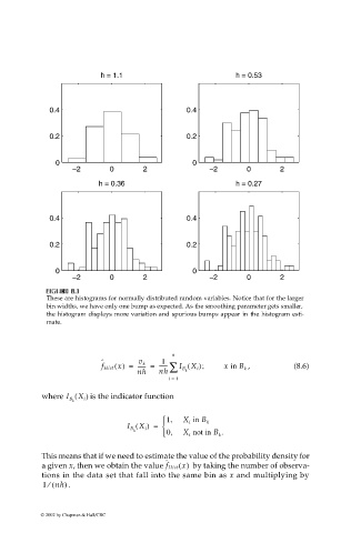
These are histograms for normally distributed random variables. Notice that for the larger
bin widths, we have only one bump as expected. As the smoothing parameter gets smaller,
the histogram displays more variation and spurious bumps appear in the histogram esti-
mate.
n
ˆ v k 1
(
f Hist x() = ------ = ------ ∑ I B X i ); x in B k , (8.6)
nh nh k
i = 1
where I B X i ) is the indicator function
(
k
 1, X i in B k
I ( X ) = 
B
 X not in B .
k i 0,
i
k
This means that if we need to estimate the value of the probability density for
ˆ
a given x, then we obtain the value f Hist x() by taking the number of observa-
tions in the data set that fall into the same bin as x and multiplying by
⁄
1 ( nh) .

© 2002 by Chapman & Hall/CRC