Page 274 - Computational Statistics Handbook with MATLAB

Chapter 8: Probability Density Estimation 263

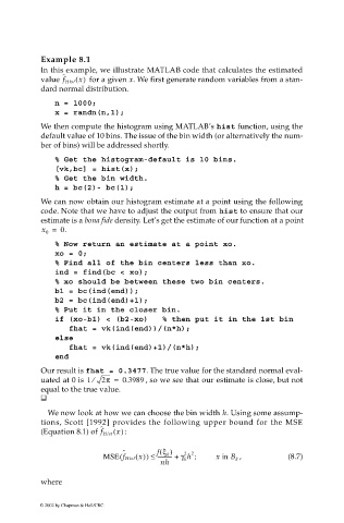
Example 8.1
In this example, we illustrate MATLAB code that calculates the estimated
ˆ
value f Hist x() for a given x. We first generate random variables from a stan-
dard normal distribution.
n = 1000;
x = randn(n,1);

We then compute the histogram using MATLAB’s hist function, using the
default value of 10 bins. The issue of the bin width (or alternatively the num-
ber of bins) will be addressed shortly.

% Get the histogram-default is 10 bins.
[vk,bc] = hist(x);
% Get the bin width.
h = bc(2)- bc(1);

We can now obtain our histogram estimate at a point using the following
code. Note that we have to adjust the output from hist to ensure that our
estimate is a bona fide density. Let’s get the estimate of our function at a point
x 0 = 0.
% Now return an estimate at a point xo.
xo = 0;
% Find all of the bin centers less than xo.
ind = find(bc < xo);
% xo should be between these two bin centers.
b1 = bc(ind(end));
b2 = bc(ind(end)+1);
% Put it in the closer bin.
if (xo-b1) < (b2-xo) % then put it in the 1st bin
fhat = vk(ind(end))/(n*h);
else
fhat = vk(ind(end)+1)/(n*h);
end
Our result is fhat = 0.3477. The true value for the standard normal eval-
uated at 0 is 1 ⁄ 2π = 0.3989 , so we see that our estimate is close, but not
equal to the true value.

We now look at how we can choose the bin width h. Using some assump-
tions, Scott [1992] provides the following upper bound for the MSE
ˆ
(Equation 8.1) of f Hist x() :
()
2
2
MSE f Hist x()( ˆ ) ≤ f ξ k γ k h ; x in B k , (8.7)
----------- +
nh
where

© 2002 by Chapman & Hall/CRC