Page 271 - Computational Statistics Handbook with MATLAB

260 Computational Statistics Handbook with MATLAB

We present three main methods of semi-parametric and nonparametric den-
sity estimation and their variants: histograms, kernel density estimates, and
finite mixtures.
In the remainder of this section, we cover some ways to measure the error
in functions as background to what follows. Then, in Section 8.2, we present
various histogram based methods for probability density estimation. There
we cover optimal bin widths for univariate and multivariate histograms, the
frequency polygons, and averaged shifted histograms. Section 8.3 contains a
discussion of kernel density estimation, both univariate and multivariate. In
Section 8.4, we describe methods that model the probability density as a finite
(less than n) sum of component densities. As usual, we conclude with
descriptions of available MATLAB code and references to the topics covered
in the chapter.
Before we can describe the various density estimation methods, we need to
provide a little background on measuring the error in functions. We briefly
present two ways to measure the error between the true function and the esti-
mate of the function. These are called the mean integrated squared error
(MISE) and the mean integrated absolute error (MIAE). Much of the under-
lying theory for choosing optimal parameters for probability density estima-
tion is based on these concepts.
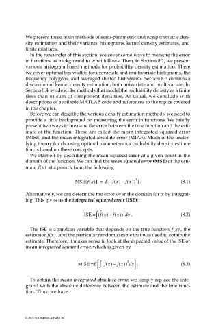
We start off by describing the mean squared error at a given point in the
domain of the function. We can find the mean squared error (MSE) of the esti-
ˆ
mate f x() at a point x from the following
ˆ
ˆ
( [
[
MSE f x()] = Ef x() – fx()) 2 . ] (8.1)
Alternatively, we can determine the error over the domain for x by integrat-
ing. This gives us the integrated squared error (ISE):
∫
ISE = ( ˆ f x() – fx()) 2 . x d (8.2)

The ISE is a random variable that depends on the true function f x() , the
estimator f x() , and the particular random sample that was used to obtain the
ˆ
estimate. Therefore, it makes sense to look at the expected value of the ISE or
mean integrated squared error, which is given by

2
MISE =E ∫ ( ˆ f x() – fx()) xd . (8.3)

To obtain the mean integrated absolute error, we simply replace the inte-
grand with the absolute difference between the estimate and the true func-
tion. Thus, we have

© 2002 by Chapman & Hall/CRC